Convex Hull Computation with convhull

Compute the convex hull of sets of points in 2-D and 3-D by using the convhull function.

The convhull and convhulln functions take a set of points and output the indices of the points that lie on the boundary of the convex hull. The point index-based representation of the convex hull supports plotting and convenient data access. The following examples illustrate the computation and representation of the convex hull.

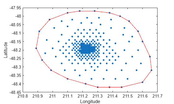
Load the data for a 2-D point set from the seamount dataset.

load seamount

Compute the convex hull of the point set.

K = convhull(x,y);

K represents the indices of the points arranged in a counter-clockwise cycle around the convex hull.

Plot the data and its convex hull.

plot(x,y,".",MarkerSize=12)
xlabel("Longitude")
ylabel("Latitude")
hold on

plot(x(K),y(K),"r")

Add point labels to the points on the convex hull to observe the structure of K.

[K,A] = convhull(x,y);

convhull can compute the convex hull of both 2-D and 3-D point sets. You can reuse the seamount dataset to illustrate the computation of the 3-D convex hull.

Include the seamount z-coordinate data elevations.

close(gcf)
K = convhull(x,y,z);

In 3-D the boundary of the convex hull, K, is represented by a triangulation. This is a set of triangular facets in matrix format that is indexed with respect to the point array. Each row of the matrix K represents a triangle.

Since the boundary of the convex hull is represented as a triangulation, you can use the triangulation plotting function trisurf.

trisurf(K,x,y,z,FaceColor="cyan")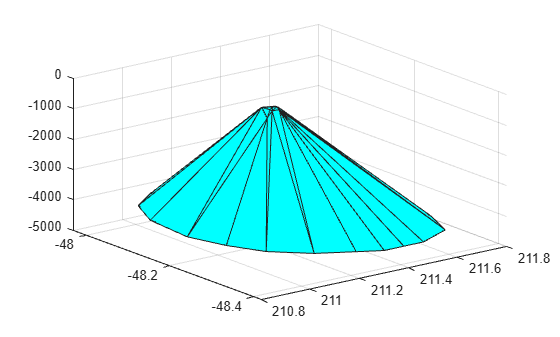

The volume bounded by the 3-D convex hull can optionally be returned by convhull, the syntax is as follows.

[K,V] = convhull(x,y,z);

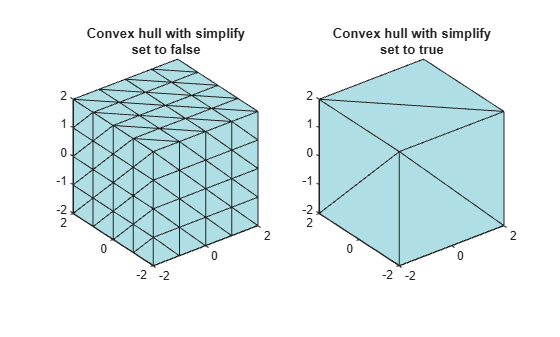
The convhull function also provides the option of simplifying the representation of the convex hull by removing vertices that do not contribute to the area or volume. For example, if boundary facets of the convex hull are collinear or coplanar, you can merge them to give a more concise representation. The following example illustrates use of this option.

[x,y,z] = meshgrid(-2:1:2,-2:1:2,-2:1:2);
x = x(:);
y = y(:); 
z = z(:);

K1 = convhull(x,y,z);
subplot(1,2,1)
defaultFaceColor  = [0.6875 0.8750 0.8984];
trisurf(K1,x,y,z,FaceColor=defaultFaceColor)
axis equal
title(sprintf("Convex hull with simplify\nset to false"))

K2 = convhull(x,y,z,Simplify=true);
subplot(1,2,2)
trisurf(K2,x,y,z,FaceColor=defaultFaceColor)
axis equal
title(sprintf("Convex hull with simplify\nset to true"))

MATLAB provides the convhulln function to support the computation of convex hulls and hypervolumes in higher dimensions. Though convhulln supports N-D, problems in more than 10 dimensions present challenges due to the rapidly growing memory requirements.

The convhull function is superior to convhulln in 2-D and 3-D as it is more robust and gives better performance.