Solve System of PDEs
This example shows how to formulate, compute, and plot the solution to a system of two partial differential equations.
Consider the system of PDEs
(The function is used as a shorthand.)
The equation holds on the interval for times . The initial conditions are
The boundary conditions are
To solve this equation in MATLAB®, you need to code the equation, the initial conditions, and the boundary conditions, then select a suitable solution mesh before calling the solver pdepe. You either can include the required functions as local functions at the end of a file (as done here), or save them as separate, named files in a directory on the MATLAB path.
Code Equation
Before you can code the equation, you need to make sure that it is in the form that the pdepe solver expects:
In this form, the PDE coefficients are matrix-valued and the equation becomes
So the values of the coefficients in the equation are
(diagonal values only)
Now you can create a function to code the equation. The function should have the signature [c,f,s] = pdefun(x,t,u,dudx):
xis the independent spatial variable.tis the independent time variable.uis the dependent variable being differentiated with respect toxandt. It is a two-element vector whereu(1)is andu(2)is .dudxis the partial spatial derivative . It is a two-element vector wheredudx(1)is anddudx(2)is .The outputs
c,f, andscorrespond to coefficients in the standard PDE equation form expected bypdepe.
As a result, the equations in this example can be represented by the function:
function [c,f,s] = pdefun(x,t,u,dudx)
c = [1; 1];
f = [0.024; 0.17] .* dudx;
y = u(1) - u(2);
F = exp(5.73*y)-exp(-11.47*y);
s = [-F; F];
end
(Note: All functions are included as local functions at the end of the example.)
Code Initial Conditions
Next, write a function that returns the initial condition. The initial condition is applied at the first time value and provides the value of for any value of x. The number of initial conditions must equal the number of equations, so for this problem there are two initial conditions. Use the function signature u0 = pdeic(x) to write the function.
The initial conditions are
The corresponding function is
function u0 = pdeic(x)
u0 = [1; 0];
end
Code Boundary Conditions
Now, write a function that evaluates the boundary conditions
For problems posed on the interval , the boundary conditions apply for all and either or . The standard form for the boundary conditions expected by the solver is
Written in this form, the boundary conditions for the partial derivatives of need to be expressed in terms of the flux . So the boundary conditions for this problem are
For , the equation is
The coefficients are:
Likewise, for the equation is
The coefficients are:
The boundary function should use the function signature [pl,ql,pr,qr] = pdebc(xl,ul,xr,ur,t):
The inputs
xlandulcorrespond to and for the left boundary.The inputs
xrandurcorrespond to and for the right boundary.tis the independent time variable.The outputs
plandqlcorrespond to and for the left boundary ( for this problem).The outputs
prandqrcorrespond to and for the right boundary ( for this problem).
The boundary conditions in this example are represented by the function:
function [pl,ql,pr,qr] = pdebc(xl,ul,xr,ur,t)
pl = [0; ul(2)];
ql = [1; 0];
pr = [ur(1)-1; 0];
qr = [0; 1];
end
Select Solution Mesh
The solution to this problem changes rapidly when is small. Although pdepe selects a time step that is appropriate to resolve the sharp changes, to see the behavior in the output plots you need to select appropriate output times. For the spatial mesh, there are boundary layers in the solution at both ends of , so you need to specify mesh points there to resolve the sharp changes.
x = [0 0.005 0.01 0.05 0.1 0.2 0.5 0.7 0.9 0.95 0.99 0.995 1];
t = [0 0.005 0.01 0.05 0.1 0.5 1 1.5 2];
Solve Equation
Finally, solve the equation using the symmetry , the PDE equation, the initial conditions, the boundary conditions, and the meshes for and .
m = 0;
sol = pdepe(m,@pdefun,@pdeic,@pdebc,x,t);
pdepe returns the solution in a 3-D array sol, where sol(i,j,k) approximates the kth component of the solution evaluated at t(i) and x(j). Extract each solution component into a separate variable.
u1 = sol(:,:,1);
u2 = sol(:,:,2);
Plot Solution
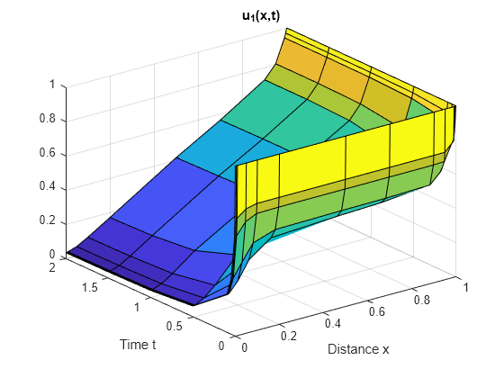
Create surface plots of the solutions for and plotted at the selected mesh points for and .
surf(x,t,u1)
title('u_1(x,t)')
xlabel('Distance x')
ylabel('Time t')
surf(x,t,u2)
title('u_2(x,t)')
xlabel('Distance x')
ylabel('Time t')

Local Functions
Listed here are the local helper functions that the PDE solver pdepe calls to calculate the solution. Alternatively, you can save these functions as their own files in a directory on the MATLAB path.
function [c,f,s] = pdefun(x,t,u,dudx) % Equation to solve
c = [1; 1];
f = [0.024; 0.17] .* dudx;
y = u(1) - u(2);
F = exp(5.73*y)-exp(-11.47*y);
s = [-F; F];
end
% ---------------------------------------------
function u0 = pdeic(x) % Initial Conditions
u0 = [1; 0];
end
% ---------------------------------------------
function [pl,ql,pr,qr] = pdebc(xl,ul,xr,ur,t) % Boundary Conditions
pl = [0; ul(2)];
ql = [1; 0];
pr = [ur(1)-1; 0];
qr = [0; 1];
end
% ---------------------------------------------