thetaregion

Filled wedge in polar coordinates

Since R2024a

Syntax

thetaregion(theta1,theta2)

thetaregion(T)

thetaregion(___,Name=Value)

thetaregion(pax,___)

pr = thetaregion(___)

Description

thetaregion(theta1,theta2) creates a filled wedge between the two specified angles in the current (polar) axes. To create one filled wedge, specify theta1 and theta2 as scalars. To create multiple filled wedges, specify theta1 and theta2 as vectors of the same length.

thetaregion(T) specifies multiple wedges as a matrix. To create n wedges, specify T as a 2-by-n or n-by-2 matrix containing the bounding angles for each wedge.

thetaregion(___,Name=Value) specifies properties for the filled wedge using one or more name-value arguments. If you create multiple wedges, the property values apply to all of the wedges. Specify the name-value arguments after all other inputs. For example, create a yellow wedge using thetaregion(0,pi/2,FaceColor="yellow"). For a list of properties, see PolarRegion Properties.

thetaregion(pax,___) specifies the target polar axes for the filled wedge. Specify pax as the first argument in any of the previous syntaxes.

pr = thetaregion(___) returns one or more PolarRegion objects. Use pr to set properties of the filled wedges after creating them. For a list of properties, see PolarRegion Properties.

Examples

Create Filled Wedge with Tick Labels in Radians

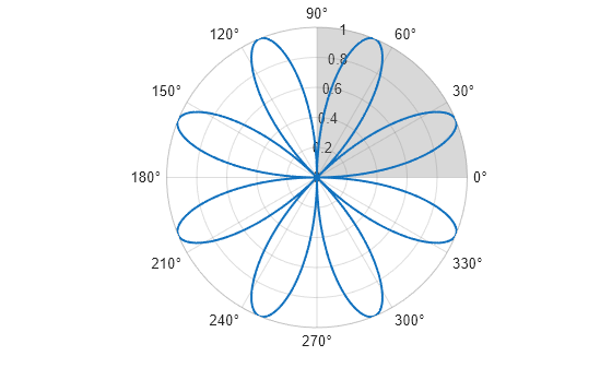
Create a polar plot. Then create a filled wedge between the angles 0 and pi/2.

% Create polar plot
theta = 0:0.01:2*pi;
rho = 2*sin(2*theta).*cos(2*theta);
polarplot(theta,rho,LineWidth=1.5)

% Create wedge
theta1 = 0;
theta2 = pi/2;
thetaregion(theta1,theta2)

Change the theta-axis units to radians by setting the ThetaAxisUnits property.

pax = gca;
pax.ThetaAxisUnits = "radians";

Create Multiple Filled Wedges

Create three filled wedges by specifying the theta values as three-element vectors.

theta1 = [pi/3 7*pi/6 10*pi/6];
theta2 = [pi/2 4*pi/3 11*pi/6];
thetaregion(theta1,theta2)

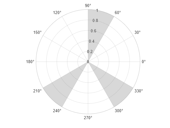
Alternatively, specify one 2-by-3 matrix of theta values.

figure
T = [pi/3 7*pi/6 10*pi/6; pi/2 4*pi/3 11*pi/6];
thetaregion(T)

Customize Fill Color and Boundary Lines

You can specify PolarRegion properties, such as face color and boundary line width and color, by specifying one or more name-value arguments when you call thetaregion. Alternatively, you can set properties of the PolarRegion object after creating it.

For example, create two green filled wedges: one in the first (upper-right) quadrant and the other in the third (lower-left) quadrant. Specify an output argument to store the PolarRegion objects so that you can modify them later.

theta1 = [0 pi];
theta2 = [pi/2 3*pi/2];
tr = thetaregion(theta1,theta2,FaceColor="g");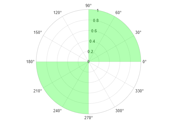

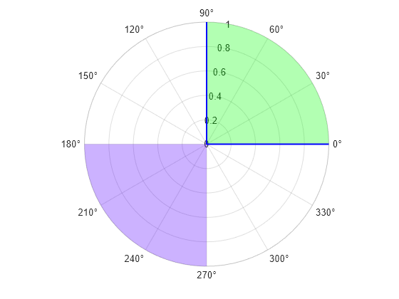
Change the color of the wedge in the third quadrant to a shade of purple by setting the FaceColor property to a hexadecimal color code. Then display thick boundary lines on the wedge in the first quadrant by setting the EdgeColor property to a value other than "none" and LineWidth property to 1.5 points.

% Set color of wedge in third quadrant
tr(2).FaceColor = "#5500FF";

% Set boundary color and line thickness in first quadrant
tr(1).EdgeColor = "b";
tr(1).LineWidth = 1.5;

Match Wedge Color to Plot Color

Plot a blue and a red cardioid.

theta = linspace(0,2*pi);
rho1 = 1-cos(theta);
rho2 = 1-cos(theta+pi);

% Blue cardioid
cardioid1 = polarplot(theta,rho1,LineWidth=1.5);
hold on

% Red cardioid
cardioid2 = polarplot(theta,rho2,LineWidth=1.5);

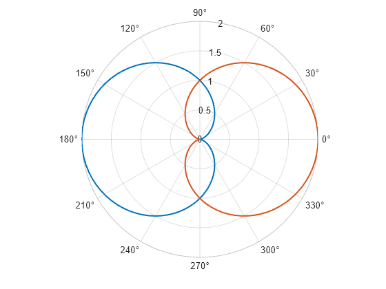
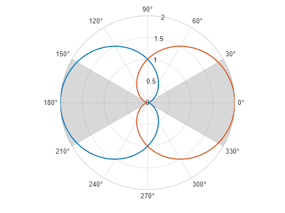
Create wedges that highlight specific regions of each cardioid.

theta1 = 5*pi/6;
theta2 = 7*pi/6;
wedge1 = thetaregion(theta1,theta2);

theta3 = 11*pi/6;
theta4 = 13*pi/6;
wedge2 = thetaregion(theta3,theta4);

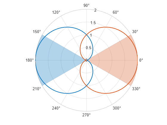
Match each wedge color to the corresponding cardioid by setting the SeriesIndex property of the wedge to the SeriesIndex property of the cardioid.

wedge1.SeriesIndex = cardioid1.SeriesIndex;
wedge2.SeriesIndex = cardioid2.SeriesIndex;

Move Wedge on Top of Plot

To move a wedge on top of a plot, set the Layer property of the PolarRegion object to "top". For example, plot a polar rose and add a filled wedge. When you create the wedge, specify a custom face color and a transparency value so that you can see that the rose is on top of the wedge.

% Plot polar rose
theta = 0:0.01:2*pi;
rho = sin(2*theta).*cos(2*theta);
polarplot(theta,rho,LineWidth=1.5)

% Add filled wedge
theta1 = 0;
theta2 = pi/4;
tr = thetaregion(theta1,theta2,FaceColor=[0.8 0.8 0.8],FaceAlpha=0.7);

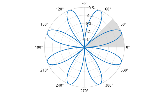
Move the filled wedge on top of the rose by setting the Layer property to "top".

tr.Layer = "top";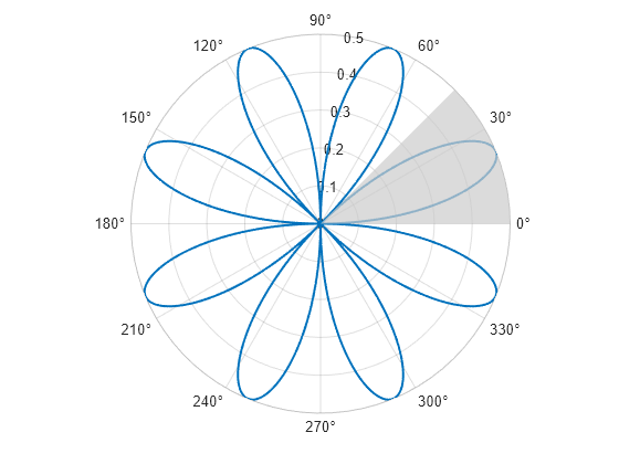

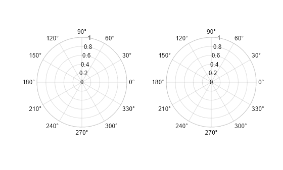
Create Filled Wedges in Different Axes

To create filled wedges in different polar axes within the same figure, create a tiled chart layout. In this case, create two axes that each contain a filled wedge.

Use the tiledlayout function to create a 1-by-2 tiled chart layout t. Use the polaraxes function to create each PolarAxes object. By default, both objects occupy the first tile. Move the second PolarAxes object to the second tile by setting the Layout.Tile property.

t = tiledlayout(1,2);
pax1 = polaraxes(t);
pax2 = polaraxes(t);
pax2.Layout.Tile = 2;

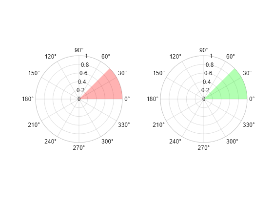
Create a red wedge in the first polar axes, and create a green wedge in the second polar axes. Specify the PolarAxes object that you want to plot into as the first argument when you call thetaregion.

theta1 = 0;
theta2 = pi/4;
thetaregion(pax1,theta1,theta2,FaceColor="r")
thetaregion(pax2,theta1,theta2,FaceColor="g")

Input Arguments

theta1,theta2 — Bounding angles (in radians)

pair of scalars | pair of vectors

Bounding angles (in radians), specified as a pair of scalars or a pair of vectors. To create one filled wedge, specify theta1 and theta2 as scalars. To create multiple filled wedges, specify vectors of equal length. You can specify the angles in any order. Thus, thetaregion(0,pi/2) and thetaregion(pi/2,0) produce the same result.

To create a circle that spans all theta values, specify one of the angles as Inf.

If you specify an angle as a NaN value, no region appears for that angle.

Example: thetaregion(pi/4,pi/2) creates a filled wedge theta=pi/4 to theta=pi/2.

Example: thetaregion([0 pi/4],[pi/6 pi/2]) creates two filled wedges: one from theta=0 to theta=pi/6 and the other from theta=pi/4 to theta=pi/2.

Data Types: single | double

T — Bounding angles for multiple wedges

2-by-n matrix | n-by-2 matrix

Bounding angles for multiple wedges, specified as a 2-by-n or n-by-2 matrix, where n is the number of wedges. If you specify a 2-by-2 matrix, each column of the matrix corresponds to a wedge.

To create a circle that spans all theta values, specify one of the angles as Inf.

If any angles are NaN values, no region appears for those angles.

Example: thetaregion([0 pi/4; pi/6 pi/2]) creates two filled wedges: one from theta=0 to theta=pi/6, and the other from theta=pi/4 to theta=pi/2.

Data Types: single | double

pax — Target polar axes

PolarAxes object

Target polar axes for the filled wedge, specified as a PolarAxes object. Use this argument if you want to create the filled wedge in a specific PolarAxes object instead of the current axes.

Name-Value Arguments

Specify optional pairs of arguments as Name1=Value1,...,NameN=ValueN, where Name is the argument name and Value is the corresponding value. Name-value arguments must appear after other arguments, but the order of the pairs does not matter.

Example: thetaregion(0,pi/2,FaceColor="yellow") creates a yellow filled wedge.

Note

The properties listed here are only a subset. For a complete list, see PolarRegion Properties.

FaceColor — Fill color

RGB triplet | hexadecimal color code | "r" | "g" | "b" | ...

Fill color, specified as an RGB triplet, a hexadecimal color code, or a color name.

For a custom color, specify an RGB triplet or a hexadecimal color code.

• An RGB triplet is a three-element row vector whose elements specify the intensities of the red, green, and blue components of the color. The intensities must be in the range [0,1], for example, [0.4 0.6 0.7].

• A hexadecimal color code is a string scalar or character vector that starts with a hash symbol (#) followed by three or six hexadecimal digits, which can range from 0 to F. The values are not case sensitive. Therefore, the color codes "#FF8800", "#ff8800", "#F80", and "#f80" are equivalent.

Alternatively, you can specify some common colors by name. This table lists the named color options, the equivalent RGB triplets, and the hexadecimal color codes.

Color Name	Short Name	RGB Triplet	Hexadecimal Color Code	Appearance
"red"	"r"	[1 0 0]	"#FF0000"
"green"	"g"	[0 1 0]	"#00FF00"
"blue"	"b"	[0 0 1]	"#0000FF"
"cyan"	"c"	[0 1 1]	"#00FFFF"
"magenta"	"m"	[1 0 1]	"#FF00FF"
"yellow"	"y"	[1 1 0]	"#FFFF00"
"black"	"k"	[0 0 0]	"#000000"
"white"	"w"	[1 1 1]	"#FFFFFF"
"none"	Not applicable	Not applicable	Not applicable	No color

This table lists the default color palettes for plots in the light and dark themes.

Palette	Palette Colors
"gem" — Light theme default Before R2025a: Most plots use these colors by default.
"glow" — Dark theme default

You can get the RGB triplets and hexadecimal color codes for these palettes using the orderedcolors and rgb2hex functions. For example, get the RGB triplets for the "gem" palette and convert them to hexadecimal color codes.

RGB = orderedcolors("gem");
H = rgb2hex(RGB);

Before R2023b: Get the RGB triplets using RGB = get(groot,"FactoryAxesColorOrder").

Before R2024a: Get the hexadecimal color codes using H = compose("#%02X%02X%02X",round(RGB*255)).

EdgeColor — Boundary line color

"none" (default) | RGB triplet | hexadecimal color code | "r" | "g" | "b" | ...

Boundary line color, specified as an RGB triplet, a hexadecimal color code, or a color name.

For a custom color, specify an RGB triplet or a hexadecimal color code.

• An RGB triplet is a three-element row vector whose elements specify the intensities of the red, green, and blue components of the color. The intensities must be in the range [0,1], for example, [0.4 0.6 0.7].

• A hexadecimal color code is a string scalar or character vector that starts with a hash symbol (#) followed by three or six hexadecimal digits, which can range from 0 to F. The values are not case sensitive. Therefore, the color codes "#FF8800", "#ff8800", "#F80", and "#f80" are equivalent.

Alternatively, you can specify some common colors by name. This table lists the named color options, the equivalent RGB triplets, and the hexadecimal color codes.

Color Name	Short Name	RGB Triplet	Hexadecimal Color Code	Appearance
"red"	"r"	[1 0 0]	"#FF0000"
"green"	"g"	[0 1 0]	"#00FF00"
"blue"	"b"	[0 0 1]	"#0000FF"
"cyan"	"c"	[0 1 1]	"#00FFFF"
"magenta"	"m"	[1 0 1]	"#FF00FF"
"yellow"	"y"	[1 1 0]	"#FFFF00"
"black"	"k"	[0 0 0]	"#000000"
"white"	"w"	[1 1 1]	"#FFFFFF"
"none"	Not applicable	Not applicable	Not applicable	No color

This table lists the default color palettes for plots in the light and dark themes.

Palette	Palette Colors
"gem" — Light theme default Before R2025a: Most plots use these colors by default.
"glow" — Dark theme default

You can get the RGB triplets and hexadecimal color codes for these palettes using the orderedcolors and rgb2hex functions. For example, get the RGB triplets for the "gem" palette and convert them to hexadecimal color codes.

RGB = orderedcolors("gem");
H = rgb2hex(RGB);

Before R2023b: Get the RGB triplets using RGB = get(groot,"FactoryAxesColorOrder").

Before R2024a: Get the hexadecimal color codes using H = compose("#%02X%02X%02X",round(RGB*255)).

FaceAlpha — Fill color transparency

0.3 (default) | scalar in range [0,1]

Fill color transparency, specified as a scalar in the range [0,1]. A value of 1 is opaque and 0 is completely transparent. Values between 0 and 1 are partially transparent.

LineStyle — Boundary line style

"-" (default) | "--" | ":" | "-." | "none"

Boundary line style, specified as one of the options listed in this table.

Line Style	Description	Resulting Line
"-"	Solid line
"--"	Dashed line
":"	Dotted line
"-."	Dash-dotted line
"none"	No line	No line

Version History

Introduced in R2024a