Large-Scale Constrained Linear Least-Squares, Problem-Based
This example shows how to recover a blurred image by solving a large-scale bound-constrained linear least-squares optimization problem. The example uses the problem-based approach. For the solver-based approach, see Large-Scale Constrained Linear Least-Squares, Solver-Based.
The Problem
Here is a photo of people sitting in a car having an interesting license plate.
load optdeblur
[m,n] = size(P);
mn = m*n;
figure
imshow(P);
colormap(gray);
axis off image;
title([string(m) + " x " + string(n) + " (" + string(mn) + ") pixels"])

The problem is to take a blurred version of this photo and try to deblur it. The starting image is black and white, meaning it consists of pixel values from 0 through 1 in the m x n matrix P.
Add Motion
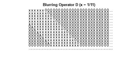
Simulate the effect of vertical motion blurring by averaging each pixel with the 5 pixels above and below. Construct a sparse matrix D to blur with a single matrix multiply.
blur = 5;
mindex = 1:mn;
nindex = 1:mn;
for i = 1:blur
  mindex=[mindex i+1:mn 1:mn-i];
  nindex=[nindex 1:mn-i i+1:mn];
end
D = sparse(mindex,nindex,1/(2*blur+1));
Draw a picture of D.
cla
axis off ij
xs = 31;
ys = 15;
xlim([0,xs+1]);
ylim([0,ys+1]);
[ix,iy] = meshgrid(1:(xs-1),1:(ys-1));
l = abs(ix-iy) <= blur;
text(ix(l),iy(l),"x")
text(ix(~l),iy(~l),"0")
text(xs*ones(ys,1),1:ys,"...");
text(1:xs,ys*ones(xs,1),"...");
title("Blurring Operator D (x = 1/11)")
Multiply the image P by the matrix D to create a blurred image G.
G = D*(P(:));
figure
imshow(reshape(G,m,n));

The image is much less distinct; you can no longer read the license plate.
Deblurred Image
To deblur, suppose that you know the blurring operator D. How well can you remove the blur and recover the original image P?
The simplest approach is to solve a least squares problem for x:
subject to .
This problem takes the blurring matrix D as given, and tries to find the x that makes Dx closest to G = DP. In order for the solution to represent sensible pixel values, restrict the solution to be from 0 through 1.
x = optimvar("x",mn,LowerBound=0,UpperBound=1);
expr = D*x-G;
objec = expr'*expr;
blurprob = optimproblem(Objective=objec);
sol = solve(blurprob);
Solving problem using quadprog. Minimum found that satisfies the constraints. Optimization completed because the objective function is non-decreasing in feasible directions, to within the value of the optimality tolerance, and constraints are satisfied to within the value of the constraint tolerance. <stopping criteria details>
xpic = reshape(sol.x,m,n);
figure
imshow(xpic)
title("Deblurred Image")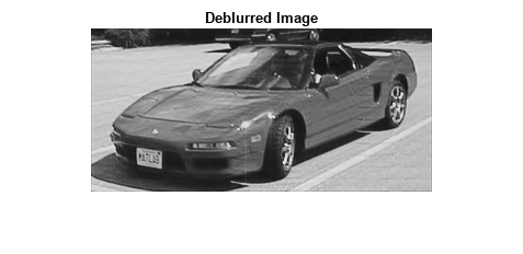
The deblurred image is much clearer than the blurred image. You can once again read the license plate. However, the deblurred image has some artifacts, such as horizontal bands in the lower-right pavement region. Perhaps these artifacts can be removed by a regularization.
Regularization
Regularization is a way to smooth the solution. There are many regularization methods. For a simple approach, add a term to the objective function as follows:
subject to .
The term makes the resulting quadratic problem more stable. Take and solve the problem again.
addI = speye(mn); expr2 = (D + 0.02*addI)*x - G; objec2 = expr2'*expr2; blurprob2 = optimproblem(Objective=objec2); sol2 = solve(blurprob2);
Solving problem using quadprog.

Minimum found that satisfies the constraints.

Optimization completed because the objective function is non-decreasing in
feasible directions, to within the value of the optimality tolerance,
and constraints are satisfied to within the value of the constraint tolerance.

<stopping criteria details>
xpic2 = reshape(sol2.x,m,n);
figure
imshow(xpic2)
title("Deblurred Regularized Image")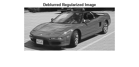
Apparently, this simple regularization does not remove the artifacts.