La traducción de esta página aún no se ha actualizado a la versión más reciente. Haga clic aquí para ver la última versión en inglés.

Ajuste de datos no lineales

Este ejemplo muestra cómo ajustar una función no lineal a los datos utilizando varios algoritmos de Optimization Toolbox™.

Configuración de problemas

Considere los siguientes datos:

Data = ...
  [0.0000    5.8955
   0.1000    3.5639
   0.2000    2.5173
   0.3000    1.9790
   0.4000    1.8990
   0.5000    1.3938
   0.6000    1.1359
   0.7000    1.0096
   0.8000    1.0343
   0.9000    0.8435
   1.0000    0.6856
   1.1000    0.6100
   1.2000    0.5392
   1.3000    0.3946
   1.4000    0.3903
   1.5000    0.5474
   1.6000    0.3459
   1.7000    0.1370
   1.8000    0.2211
   1.9000    0.1704
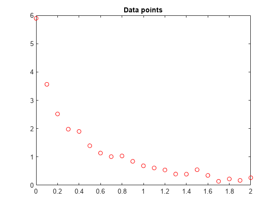
   2.0000    0.2636];

Representemos estos puntos de datos.

t = Data(:,1);
y = Data(:,2);
% axis([0 2 -0.5 6])
% hold on
plot(t,y,'ro')
title('Data points')

% hold off

Nos gustaría ajustar la función

y = c(1)*exp(-lam(1)*t) + c(2)*exp(-lam(2)*t)

a los datos.

Enfoque de solución utilizando lsqcurvefit

La función lsqcurvefit resuelve este tipo de problema fácilmente.

Para comenzar, defina los parámetros en términos de una variable x:

x(1) = c(1)

x(2) = lam(1)

x(3) = c(2)

x(4) = lam(2)

Después, defina la curva como una función de los parámetros x y los datos t:

F = @(x,xdata)x(1)*exp(-x(2)*xdata) + x(3)*exp(-x(4)*xdata);

De forma arbitraria, hemos configurado nuestro punto inicial x0 de la siguiente manera: c(1) = 1, lam(1) = 1, c(2) = 1, lam(2) = 0:

x0 = [1 1 1 0];

Ejecutamos el solver y representamos el ajuste resultante.

[x,resnorm,~,exitflag,output] = lsqcurvefit(F,x0,t,y)

Local minimum possible.

lsqcurvefit stopped because the final change in the sum of squares relative to 
its initial value is less than the value of the function tolerance.

x = 1×4

    3.0068   10.5869    2.8891    1.4003

resnorm = 0.1477

exitflag = 3

output = struct with fields:
    firstorderopt: 7.8830e-06
       iterations: 6
        funcCount: 35
     cgiterations: 0
        algorithm: 'trust-region-reflective'
         stepsize: 0.0096
          message: 'Local minimum possible....'

hold on
plot(t,F(x,t))
hold off

Enfoque de solución utilizando fminunc

Para resolver el problema utilizando fminunc, establecemos la función objetivo como la suma de cuadrados de los valores residuales.

Fsumsquares = @(x)sum((F(x,t) - y).^2);
opts = optimoptions('fminunc','Algorithm','quasi-newton');
[xunc,ressquared,eflag,outputu] = ...
    fminunc(Fsumsquares,x0,opts)

Local minimum found.

Optimization completed because the size of the gradient is less than
the value of the optimality tolerance.

xunc = 1×4

    2.8890    1.4003    3.0069   10.5862

ressquared = 0.1477

eflag = 1

outputu = struct with fields:
       iterations: 30
        funcCount: 185
         stepsize: 0.0017
     lssteplength: 1
    firstorderopt: 2.9662e-05
        algorithm: 'quasi-newton'
          message: 'Local minimum found....'

Tenga en cuenta que fminunc ha encontrado la misma solución que lsqcurvefit, pero ha necesitado muchas más evaluaciones para hacerlo. Los parámetros para fminunc están en el orden inverso a los parámetros para lsqcurvefit; el lam mayor es lam(2), no lam(1). No resulta sorprendente, ya que el orden de variables es arbitrario.

fprintf(['There were %d iterations using fminunc,' ...
    ' and %d using lsqcurvefit.\n'], ...
    outputu.iterations,output.iterations)

There were 30 iterations using fminunc, and 6 using lsqcurvefit.

fprintf(['There were %d function evaluations using fminunc,' ...
    ' and %d using lsqcurvefit.'], ...
    outputu.funcCount,output.funcCount)

There were 185 function evaluations using fminunc, and 35 using lsqcurvefit.

Dividir los problemas lineales y no lineales

Tenga en cuenta que el problema de ajuste es lineal en los parámetros c(1) y c(2). Esto significa que, para cualquier valor de lam(1) y lam(2), podemos utilizar el operador de barra invertida con el propósito de encontrar los valores de c(1) and c(2) que resuelvan el problema de mínimos cuadrados.

Ahora, rehacemos el problema como problema de dos dimensiones y buscamos los mejores valores de lam(1) y lam(2). Los valores de c(1) y c(2) se calculan en cada paso utilizando el operador de barra invertida tal y como se ha descrito anteriormente.

type fitvector

function yEst = fitvector(lam,xdata,ydata)
%FITVECTOR  Used by DATDEMO to return value of fitting function.
%   yEst = FITVECTOR(lam,xdata) returns the value of the fitting function, y
%   (defined below), at the data points xdata with parameters set to lam.
%   yEst is returned as a N-by-1 column vector, where N is the number of
%   data points.
%
%   FITVECTOR assumes the fitting function, y, takes the form
%
%     y =  c(1)*exp(-lam(1)*t) + ... + c(n)*exp(-lam(n)*t)
%
%   with n linear parameters c, and n nonlinear parameters lam.
%
%   To solve for the linear parameters c, we build a matrix A
%   where the j-th column of A is exp(-lam(j)*xdata) (xdata is a vector).
%   Then we solve A*c = ydata for the linear least-squares solution c,
%   where ydata is the observed values of y.

A = zeros(length(xdata),length(lam));  % build A matrix
for j = 1:length(lam)
   A(:,j) = exp(-lam(j)*xdata);
end
c = A\ydata; % solve A*c = y for linear parameters c
yEst = A*c; % return the estimated response based on c

Resuelva el problema utilizando lsqcurvefit, comenzando por un punto inicial de dos dimensiones lam(1), lam(2):

x02 = [1 0];
F2 = @(x,t) fitvector(x,t,y);

[x2,resnorm2,~,exitflag2,output2] = lsqcurvefit(F2,x02,t,y)

Local minimum possible.

lsqcurvefit stopped because the final change in the sum of squares relative to 
its initial value is less than the value of the function tolerance.

x2 = 1×2

   10.5861    1.4003

resnorm2 = 0.1477

exitflag2 = 3

output2 = struct with fields:
    firstorderopt: 4.4087e-06
       iterations: 10
        funcCount: 33
     cgiterations: 0
        algorithm: 'trust-region-reflective'
         stepsize: 0.0080
          message: 'Local minimum possible....'

La eficacia de la solución de dos dimensiones es similar a la de la solución de cuatro dimensiones:

fprintf(['There were %d function evaluations using the 2-d ' ...
    'formulation, and %d using the 4-d formulation.'], ...
    output2.funcCount,output.funcCount)

There were 33 function evaluations using the 2-d formulation, and 35 using the 4-d formulation.

El problema de división es más robusto a la conjetura inicial

Escoger un mal punto de inicio para el problema original de cuatro parámetros hace que se obtenga solución local que no es global. Escoger un punto de inicio con los mismos valores malos lam(1) y lam(2) para el problema de división de dos parámetros hace que se obtenga la solución global. Para mostrarlo, volvemos a ejecutar el problema original con un punto de inicio con el que se obtiene una solución local relativamente mala y comparamos el ajuste resultante con la solución global.

x0bad = [5 1 1 0];
[xbad,resnormbad,~,exitflagbad,outputbad] = ...
    lsqcurvefit(F,x0bad,t,y)

Local minimum possible.

lsqcurvefit stopped because the final change in the sum of squares relative to 
its initial value is less than the value of the function tolerance.

xbad = 1×4

  -22.9036    2.4792   28.0273    2.4791

resnormbad = 2.2173

exitflagbad = 3

outputbad = struct with fields:
    firstorderopt: 0.0056
       iterations: 32
        funcCount: 165
     cgiterations: 0
        algorithm: 'trust-region-reflective'
         stepsize: 0.0021
          message: 'Local minimum possible....'

hold on
plot(t,F(xbad,t),'g')
legend('Data','Global fit','Bad local fit','Location','NE')
hold off

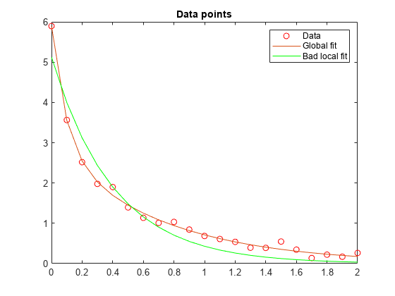
fprintf(['The residual norm at the good ending point is %f,' ...
   ' and the residual norm at the bad ending point is %f.'], ...
   resnorm,resnormbad)

The residual norm at the good ending point is 0.147723, and the residual norm at the bad ending point is 2.217300.

Temas relacionados

• Nonlinear Data-Fitting Using Several Problem-Based Approaches
• Mínimos cuadrados no lineales, sin y con matrices jacobianas
• Ajuste no lineal de curvas con lsqcurvefit

×

Abrir ejemplo

Tiene una versión modificada de este ejemplo. ¿Desea abrir este ejemplo con sus modificaciones?

No, sobrescribir la versión modificada Sí