La traducción de esta página aún no se ha actualizado a la versión más reciente. Haga clic aquí para ver la última versión en inglés.

Ajuste de datos no lineales empleando varios enfoques basados en problemas

El consejo general para la configuración de problemas de mínimos cuadrados es formular el problema de tal manera que solve reconozca que tiene un formato de mínimos cuadrados. Cuando se hace eso, solve llama internamente a lsqnonlin, que es eficiente para resolver problemas de mínimos cuadrados. Consulte Write Objective Function for Problem-Based Least Squares.

En este ejemplo se muestra la eficiencia de un solver de mínimos cuadrados comparando el rendimiento de lsqnonlin con el de fminunc en el mismo problema. Además, en el ejemplo se muestran ventajas adicionales que se pueden obtener reconociendo explícitamente y gestionando por separado las partes lineales de un problema.

Configuración de problemas

Considere los siguientes datos:

Data = ...
  [0.0000    5.8955
   0.1000    3.5639
   0.2000    2.5173
   0.3000    1.9790
   0.4000    1.8990
   0.5000    1.3938
   0.6000    1.1359
   0.7000    1.0096
   0.8000    1.0343
   0.9000    0.8435
   1.0000    0.6856
   1.1000    0.6100
   1.2000    0.5392
   1.3000    0.3946
   1.4000    0.3903
   1.5000    0.5474
   1.6000    0.3459
   1.7000    0.1370
   1.8000    0.2211
   1.9000    0.1704
   2.0000    0.2636];

Represente los puntos de datos.

t = Data(:,1);
y = Data(:,2);
plot(t,y,'ro')
title('Data points')

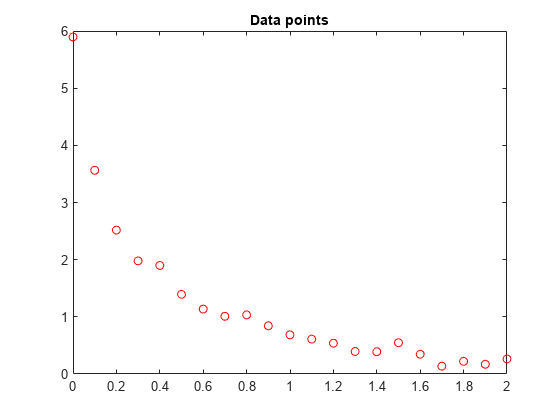
El problema consiste en ajustar la función

y = c(1)*exp(-lam(1)*t) + c(2)*exp(-lam(2)*t)

a los datos.

Enfoque de solución utilizando el solver predeterminado

Para empezar, defina variables de optimización correspondientes a la ecuación.

c = optimvar('c',2);
lam = optimvar('lam',2);

De forma arbitraria, establezca el punto inicial x0 de la forma siguiente: c(1) = 1, c(2) = 1, lam(1) = 1 y lam(2) = 0:

x0.c = [1,1];
x0.lam = [1,0];

Cree una función que calcule el valor de la respuesta en tiempos t cuando los parámetros son c y lam.

diffun = c(1)*exp(-lam(1)*t) + c(2)*exp(-lam(2)*t);

Convierta diffun en una expresión de optimización que suma los cuadrados de las diferencias entre la función y los datos y.

diffexpr = sum((diffun - y).^2);

Cree un problema de optimización con diffexpr como la función objetivo.

ssqprob = optimproblem('Objective',diffexpr);

Resuelva el problema utilizando el solver predeterminado.

[sol,fval,exitflag,output] = solve(ssqprob,x0)

Solving problem using lsqnonlin.

Local minimum possible.

lsqnonlin stopped because the final change in the sum of squares relative to 
its initial value is less than the value of the function tolerance.

sol = struct with fields:
      c: [2x1 double]
    lam: [2x1 double]

fval = 0.1477

exitflag = 
    FunctionChangeBelowTolerance

output = struct with fields:
           firstorderopt: 7.8870e-06
              iterations: 6
               funcCount: 7
            cgiterations: 0
               algorithm: 'trust-region-reflective'
                stepsize: 0.0096
                 message: 'Local minimum possible....'
            bestfeasible: []
         constrviolation: []
     objectivederivative: "forward-AD"
    constraintderivative: "closed-form"
                  solver: 'lsqnonlin'

Represente la curva resultante a partir de los valores de la solución devueltos sol.c y sol.lam.

resp = evaluate(diffun,sol);
hold on
plot(t,resp)
hold off

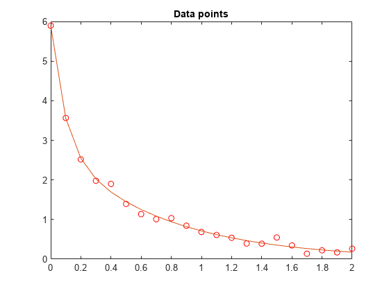
El ajuste tiene el mejor aspecto posible.

Enfoque de solución utilizando fminunc

Para resolver este problema utilizando el solver fminunc, establezca la opción 'Solver' en 'fminunc' al llamar a solve.

[xunc,fvalunc,exitflagunc,outputunc] = solve(ssqprob,x0,'Solver',"fminunc")

Solving problem using fminunc.

Local minimum found.

Optimization completed because the size of the gradient is less than
the value of the optimality tolerance.

xunc = struct with fields:
      c: [2x1 double]
    lam: [2x1 double]

fvalunc = 0.1477

exitflagunc = 
    OptimalSolution

outputunc = struct with fields:
             iterations: 30
              funcCount: 37
               stepsize: 0.0017
           lssteplength: 1
          firstorderopt: 2.9454e-05
              algorithm: 'quasi-newton'
                message: 'Local minimum found....'
    objectivederivative: "forward-AD"
                 solver: 'fminunc'

Tenga en cuenta que fminunc ha encontrado la misma solución que lsqcurvefit, pero ha necesitado muchas más evaluaciones para hacerlo. Los parámetros para fminunc están en el orden inverso a los de lsqcurvefit; el lam más amplio es lam(2), no lam(1). No resulta sorprendente, ya que el orden de variables es arbitrario.

fprintf(['There were %d iterations using fminunc,' ...
    ' and %d using lsqcurvefit.\n'], ...
    outputunc.iterations,output.iterations)

There were 30 iterations using fminunc, and 6 using lsqcurvefit.

fprintf(['There were %d function evaluations using fminunc,' ...
    ' and %d using lsqcurvefit.'], ...
    outputunc.funcCount,output.funcCount)

There were 37 function evaluations using fminunc, and 7 using lsqcurvefit.

Dividir los problemas lineales y no lineales

Tenga en cuenta que el problema de ajuste es lineal en los parámetros c(1) y c(2). Esto significa que, para cualquier valor de lam(1) y lam(2), puede utilizar el operador de barra invertida con el propósito de encontrar los valores de c(1) y c(2) que resuelvan el problema de mínimos cuadrados.

Reformule el problema como problema de dos dimensiones, buscando los mejores valores de lam(1) y lam(2). Los valores de c(1) y c(2) se calculan en cada paso utilizando el operador de barra invertida tal y como se ha descrito anteriormente. Para hacerlo, utilice la función fitvector, que realiza la operación de barra invertida para obtener c(1) y c(2) en cada iteración del solver.

type fitvector

function yEst = fitvector(lam,xdata,ydata)
%FITVECTOR  Used by DATDEMO to return value of fitting function.
%   yEst = FITVECTOR(lam,xdata) returns the value of the fitting function, y
%   (defined below), at the data points xdata with parameters set to lam.
%   yEst is returned as a N-by-1 column vector, where N is the number of
%   data points.
%
%   FITVECTOR assumes the fitting function, y, takes the form
%
%     y =  c(1)*exp(-lam(1)*t) + ... + c(n)*exp(-lam(n)*t)
%
%   with n linear parameters c, and n nonlinear parameters lam.
%
%   To solve for the linear parameters c, we build a matrix A
%   where the j-th column of A is exp(-lam(j)*xdata) (xdata is a vector).
%   Then we solve A*c = ydata for the linear least-squares solution c,
%   where ydata is the observed values of y.

A = zeros(length(xdata),length(lam));  % build A matrix
for j = 1:length(lam)
   A(:,j) = exp(-lam(j)*xdata);
end
c = A\ydata; % solve A*c = y for linear parameters c
yEst = A*c; % return the estimated response based on c

Resuelva el problema utilizando solve, empezando por un punto inicial de dos dimensiones x02.lam = [1,0]. Para hacerlo, primero convierta la función fitvector en una expresión de optimización utilizando fcn2optimexpr. Consulte Convertir una función no lineal en una expresión de optimización. Para evitar una advertencia, proporcione el tamaño de salida de la expresión resultante. Cree un nuevo problema de optimización con el objetivo como la suma de las diferencias al cuadrado entre la función convertida fitvector y los datos y.

x02.lam = x0.lam;
F2 = fcn2optimexpr(@(x) fitvector(x,t,y),lam,'OutputSize',[length(t),1]);
ssqprob2 = optimproblem('Objective',sum((F2 - y).^2));
[sol2,fval2,exitflag2,output2] = solve(ssqprob2,x02)

Solving problem using lsqnonlin.

Local minimum possible.

lsqnonlin stopped because the final change in the sum of squares relative to 
its initial value is less than the value of the function tolerance.

sol2 = struct with fields:
    lam: [2x1 double]

fval2 = 0.1477

exitflag2 = 
    FunctionChangeBelowTolerance

output2 = struct with fields:
           firstorderopt: 4.4018e-06
              iterations: 10
               funcCount: 33
            cgiterations: 0
               algorithm: 'trust-region-reflective'
                stepsize: 0.0080
                 message: 'Local minimum possible....'
            bestfeasible: []
         constrviolation: []
     objectivederivative: "finite-differences"
    constraintderivative: "closed-form"
                  solver: 'lsqnonlin'

La eficacia de la solución de dos dimensiones es similar a la de la solución de cuatro dimensiones:

fprintf(['There were %d function evaluations using the 2-d ' ...
    'formulation, and %d using the 4-d formulation.'], ...
    output2.funcCount,output.funcCount)

There were 33 function evaluations using the 2-d formulation, and 7 using the 4-d formulation.

El problema de división es más robusto a la conjetura inicial

Escoger un mal punto de inicio para el problema original de cuatro parámetros hace que se obtenga solución local que no es global. Escoger un punto de inicio con los mismos valores malos lam(1) y lam(2) para el problema de división de dos parámetros hace que se obtenga la solución global. Para mostrarlo, vuelva a ejecutar el problema original con un punto de inicio con el que se obtiene una solución local relativamente mala y compare el ajuste resultante con la solución global.

x0bad.c = [5 1];
x0bad.lam = [1 0];
[solbad,fvalbad,exitflagbad,outputbad] = solve(ssqprob,x0bad)

Solving problem using lsqnonlin.

Local minimum possible.

lsqnonlin stopped because the final change in the sum of squares relative to 
its initial value is less than the value of the function tolerance.

solbad = struct with fields:
      c: [2x1 double]
    lam: [2x1 double]

fvalbad = 2.2173

exitflagbad = 
    FunctionChangeBelowTolerance

outputbad = struct with fields:
           firstorderopt: 0.0036
              iterations: 31
               funcCount: 32
            cgiterations: 0
               algorithm: 'trust-region-reflective'
                stepsize: 0.0012
                 message: 'Local minimum possible....'
            bestfeasible: []
         constrviolation: []
     objectivederivative: "forward-AD"
    constraintderivative: "closed-form"
                  solver: 'lsqnonlin'

respbad = evaluate(diffun,solbad);
hold on
plot(t,respbad,'g')
legend('Data','Global fit','Bad local fit','Location','NE')
hold off

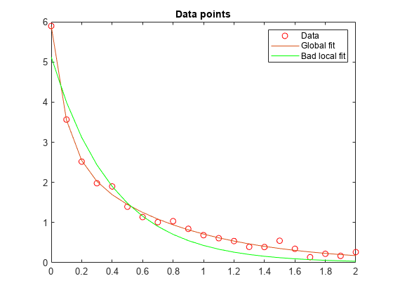
fprintf(['The residual norm at the good ending point is %f,' ...
   ' and the residual norm at the bad ending point is %f.'], ...
   fval,fvalbad)

The residual norm at the good ending point is 0.147723, and the residual norm at the bad ending point is 2.217300.

Consulte también

solve | fcn2optimexpr

Temas relacionados

• Ajuste de datos no lineales
• Flujo de trabajo de optimización basada en problemas