interpolateElectricFlux
Interpolate electric flux density in electrostatic result at arbitrary spatial locations
Syntax
Description
Dintrp = interpolateElectricFlux(electrostaticresults,xq,yq)xq and yq.
Dintrp = interpolateElectricFlux(electrostaticresults,querypoints)querypoints.
Examples
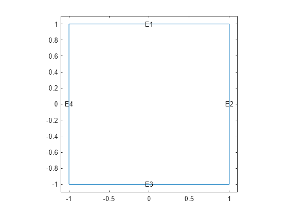
Create a square geometry and plot it with the edge labels.
R1 = [3,4,-1,1,1,-1,1,1,-1,-1]';
g = decsg(R1,'R1',('R1')');
pdegplot(g,EdgeLabels="on")
xlim([-1.1 1.1])
ylim([-1.1 1.1])

Create an femodel object for electrostatic analysis and include the geometry into the model.
model = femodel(AnalysisType="electrostatic", ...
                Geometry=g);
Specify the vacuum permittivity in the SI system of units.
model.VacuumPermittivity = 8.8541878128E-12;
Specify the relative permittivity of the material.
model.MaterialProperties = ...
    materialProperties(RelativePermittivity=1);
Apply the voltage boundary conditions on the edges of the square.
model.EdgeBC([1 3]) = edgeBC(Voltage=0);
model.EdgeBC([2 4]) = edgeBC(Voltage=1000);
Specify the charge density for the entire geometry.
model.FaceLoad = faceLoad(ChargeDensity=5E-9);
Generate the mesh.
model = generateMesh(model);
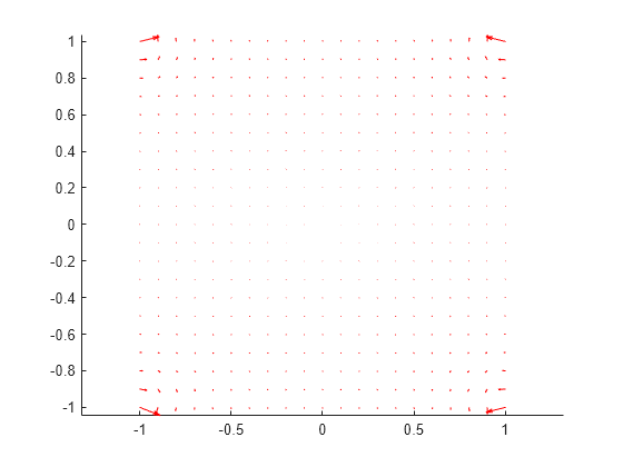
Solve the problem and plot the electric flux density.
R = solve(model);
pdeplot(R.Mesh,FlowData=[R.ElectricFluxDensity.Dx ...
                         R.ElectricFluxDensity.Dy])
axis equal

Interpolate the resulting electric flux density to a grid covering the central portion of the geometry, for x and y from -0.5 to 0.5.
v = linspace(-0.5,0.5,51);
[X,Y] = meshgrid(v);

Dintrp = interpolateElectricFlux(R,X,Y)
Dintrp =
  FEStruct with properties:

    Dx: [2601×1 double]
    Dy: [2601×1 double]
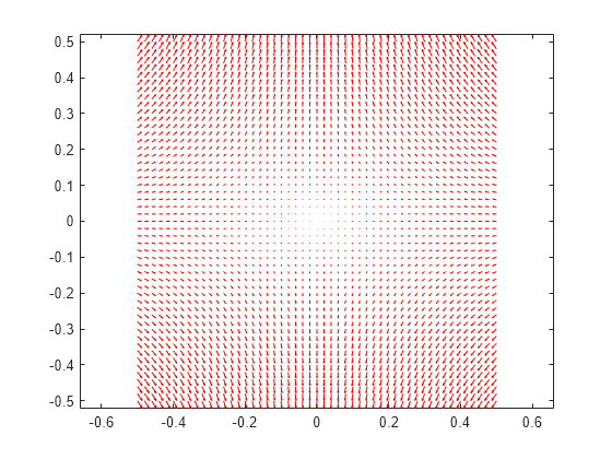
Reshape Dintrp.Dx and Dintrp.Dy and plot the resulting electric flux density.
DintrpX = reshape(Dintrp.Dx,size(X));
DintrpY = reshape(Dintrp.Dy,size(Y));

figure
quiver(X,Y,DintrpX,DintrpY,Color="red")
axis equal

Alternatively, you can specify the grid by using a matrix of query points.
querypoints = [X(:),Y(:)]';
Dintrp = interpolateElectricFlux(R,querypoints);
Create an femodel object for electrostatic analysis and include a geometry of a plate with a hole into the model.
model = femodel(AnalysisType="electrostatic", ...
                Geometry="PlateHoleSolid.stl");
Plot the geometry.
pdegplot(model.Geometry,FaceLabels="on",FaceAlpha=0.3)
Specify the vacuum permittivity in the SI system of units.
model.VacuumPermittivity = 8.8541878128E-12;
Specify the relative permittivity of the material.
model.MaterialProperties = ...
    materialProperties(RelativePermittivity=1);
Specify the charge density for the entire geometry.
model.CellLoad = cellLoad(ChargeDensity=5E-9);
Apply the voltage boundary conditions on the side faces and the face bordering the hole.
model.FaceBC(3:6) = faceBC(Voltage=0);
model.FaceBC(7) = faceBC(Voltage=1000);
Generate the mesh.
model = generateMesh(model);
Solve the problem.
R = solve(model)
R =
  ElectrostaticResults with properties:

      ElectricPotential: [4747×1 double]
          ElectricField: [1×1 FEStruct]
    ElectricFluxDensity: [1×1 FEStruct]
                   Mesh: [1×1 FEMesh]
Plot the electric flux density.
pdeplot3D(R.Mesh,FlowData=[R.ElectricFluxDensity.Dx ...
                           R.ElectricFluxDensity.Dy ...
                           R.ElectricFluxDensity.Dz])

Interpolate the resulting electric flux density to a grid covering the central portion of the geometry, for x, y, and z.
x = linspace(3,7,7);
y = linspace(0,1,7);
z = linspace(8,12,7);
[X,Y,Z] = meshgrid(x,y,z);

Dintrp = interpolateElectricFlux(R,X,Y,Z);
Reshape Dintrp.Dx, Dintrp.Dy, and Dintrp.Dz.
DintrpX = reshape(Dintrp.Dx,size(X));
DintrpY = reshape(Dintrp.Dy,size(Y));
DintrpZ = reshape(Dintrp.Dz,size(Z));
Plot the resulting electric flux density.
figure
quiver3(X,Y,Z,DintrpX,DintrpY,DintrpZ,Color="red")
view([10 10])
Input Arguments
Solution of thermal problem, specified as an ElectrostaticResults object. Create electrostaticresults
using the solve function.
x-coordinate query points, specified as a real array.
interpolateElectricFlux evaluates the electric flux density at the
2-D coordinate points [xq(i) yq(i)] or at the 3-D coordinate points
[xq(i) yq(i) zq(i)] for every i. Because of
this, xq, yq, and (if present)
zq must have the same number of entries.
interpolateElectricFlux converts the query points to column
vectors xq(:), yq(:), and (if present)
zq(:). It returns electric flux density as a column vector of the
same size. To ensure that the dimensions of the returned solution are consistent with
the dimensions of the original query points, use reshape. For
example, use DintrpX = reshape(Dintrp.Dx,size(xq)).
Example: xq = [0.5 0.5 0.75 0.75]
Data Types: double
y-coordinate query points, specified as a real array.
interpolateElectricFlux evaluates the electric flux density at the
2-D coordinate points [xq(i) yq(i)] or at the 3-D coordinate points
[xq(i) yq(i) zq(i)] for every i. Because of
this, xq, yq, and (if present)
zq must have the same number of entries.
interpolateElectricFlux converts the query points to column
vectors xq(:), yq(:), and (if present)
zq(:). It returns electric flux density as a column vector of the
same size. To ensure that the dimensions of the returned solution are consistent with
the dimensions of the original query points, use reshape. For
example, use DintrpY = reshape(Dintrp.Dy,size(yq)).
Example: yq = [1 2 0 0.5]
Data Types: double
z-coordinate query points, specified as a real array.
interpolateElectricFlux evaluates the electric flux density at the
3-D coordinate points [xq(i) yq(i) zq(i)]. Therefore,
xq, yq, and zq must have
the same number of entries.
interpolateElectricFlux converts the query points to column
vectors xq(:), yq(:), and
zq(:). It returns electric flux density values as a column vector of
the same size. To ensure that the dimensions of the returned solution are consistent
with the dimensions of the original query points, use reshape. For
example, use DintrpZ = reshape(Dintrp.Dz,size(zq)).
Example: zq = [1 1 0 1.5]
Data Types: double
Query points, specified as a real matrix with either two rows for 2-D geometry or
three rows for 3-D geometry. interpolateElectricFlux evaluates the
electric flux density at the coordinate points querypoints(:,i) for
every i, so each column of querypoints contains
exactly one 2-D or 3-D query point.
Example: For a 2-D geometry, querypoints = [0.5 0.5 0.75 0.75; 1 2 0
0.5]
Data Types: double
Output Arguments
Electric flux density at query points, returned as an FEStruct
object with the properties representing the spatial components of the electric flux
density at the query points. For query points that are outside the geometry,
Dintrp.Dx(i), Dintrp.Dy(i), and
Dintrp.Dz(i) are NaN. Properties of an
FEStruct object are read-only.
Version History
Introduced in R2021a
See Also
Objects
Functions
MATLAB Command
You clicked a link that corresponds to this MATLAB command:
Run the command by entering it in the MATLAB Command Window. Web browsers do not support MATLAB commands.
Seleccione un país/idioma
Seleccione un país/idioma para obtener contenido traducido, si está disponible, y ver eventos y ofertas de productos y servicios locales. Según su ubicación geográfica, recomendamos que seleccione: .
También puede seleccionar uno de estos países/idiomas:
Cómo obtener el mejor rendimiento
Seleccione China (en idioma chino o inglés) para obtener el mejor rendimiento. Los sitios web de otros países no están optimizados para ser accedidos desde su ubicación geográfica.
América
- América Latina (Español)
- Canada (English)
- United States (English)
Europa
- Belgium (English)
- Denmark (English)
- Deutschland (Deutsch)
- España (Español)
- Finland (English)
- France (Français)
- Ireland (English)
- Italia (Italiano)
- Luxembourg (English)
- Netherlands (English)
- Norway (English)
- Österreich (Deutsch)
- Portugal (English)
- Sweden (English)
- Switzerland
- United Kingdom (English)