applyBoundaryCondition
Add boundary condition to PDEModel container
Syntax
Description
applyBoundaryCondition(
adds a Dirichlet boundary condition to model,"dirichlet",RegionType,RegionID,Name,Value)model. The boundary
condition applies to boundary regions of type RegionType with
ID numbers in RegionID, and with arguments
r, h, u,
EquationIndex specified in the
Name,Value pairs. For Dirichlet boundary conditions,
specify either both arguments r and h, or
the argument u. When specifying u, you can
also use EquationIndex.
applyBoundaryCondition(
adds a Neumann boundary condition to model,"neumann",RegionType,RegionID,Name,Value)model. The boundary
condition applies to boundary regions of type RegionType with
ID numbers in RegionID, and with values g
and q specified in the Name,Value
pairs.
applyBoundaryCondition(
adds an individual boundary condition for each equation in a system of PDEs. The
boundary condition applies to boundary regions of type
model,"mixed",RegionType,RegionID,Name,Value)RegionType with ID numbers in
RegionID, and with values specified in the
Name,Value pairs. For mixed boundary conditions, you can use
Name,Value pairs from both Dirichlet and Neumann boundary
conditions as needed.
bc = applyBoundaryCondition(___)
Examples
Create a PDE model and geometry.
model = createpde(1);
R1 = [3,4,-1,1,1,-1,-.4,-.4,.4,.4]';
g = decsg(R1);
geometryFromEdges(model,g);
View the edge labels.
pdegplot(model,"EdgeLabels","on")
xlim([-1.2,1.2])
axis equal

Apply zero Dirichlet condition on the edge 1.
applyBoundaryCondition(model,"dirichlet", ...
                             "Edge",1,"u",0);
On other edges, apply Dirichlet condition h*u = r, where h = 1 and r = 1.
applyBoundaryCondition(model,"dirichlet", ...
                             "Edge",2:4, ...
                             "r",1,"h",1);
Create a PDE model and geometry.
model = createpde(2);
R1 = [3,4,-1,1,1,-1,-.4,-.4,.4,.4]';
g = decsg(R1);
geometryFromEdges(model,g);
View the edge labels.
pdegplot(model,"EdgeLabels","on")
xlim([-1.2,1.2])
axis equal

Apply the following Neumann boundary conditions on the edge 4.
applyBoundaryCondition(model,"neumann", ...
                             "Edge",4, ...
                             "g",[0;.123], ...
                             "q",[0;0;0;0]);
Apply both types of boundary conditions to a scalar problem. First, create a PDE model and import a simple block geometry.
model = createpde;
importGeometry(model,"Block.stl");
View the face labels.
pdegplot(model,"FaceLabels","on","FaceAlpha",0.5)

Set zero Dirichlet conditions on the narrow faces, which are labeled 1 through 4.
applyBoundaryCondition(model,"dirichlet", ...
                             "Face",1:4,"u",0);
Set Neumann boundary conditions with opposite signs on faces 5 and 6.
applyBoundaryCondition(model,"neumann", ...
                             "Face",5,"g",1);
applyBoundaryCondition(model,"neumann", ...
                             "Face",6,"g",-1);
Solve an elliptic PDE with these boundary conditions, and plot the result.
specifyCoefficients(model,"m",0,"d",0,"c",1,"a",0,"f",0);
generateMesh(model);
results = solvepde(model);
u = results.NodalSolution;
pdeplot3D(model,"ColorMapData",u)

Create a PDE model and import a simple block geometry.
model = createpde(3);
importGeometry(model,"Block.stl");
View the face labels.
pdegplot(model,"FaceLabels","on","FaceAlpha",0.5)

Set zero Dirichlet conditions on faces 1 and 2.
applyBoundaryCondition(model,"dirichlet", ...
                             "Face",1:2,"u",[0,0,0]);
Set Neumann boundary conditions with opposite signs on faces 4, 5, and 6.
applyBoundaryCondition(model,"neumann", ...
                             "Face",4:5,"g",[1;1;1]);
applyBoundaryCondition(model,"neumann", ...
                             "Face",6,"g",[-1;-1;-1]);
For face 3, apply generalized Neumann boundary condition for the first equation and Dirichlet boundary conditions for the second and third equations.
h = [0 0 0;0 1 0;0 0 1];
r = [0;3;3];
q = [1 0 0;0 0 0;0 0 0];
g = [10;0;0];
applyBoundaryCondition(model,"mixed","Face",3, ...
                       "h",h,"r",r,"g",g,"q",q);
Solve an elliptic PDE with these boundary conditions, and plot the result.
specifyCoefficients(model,"m",0,"d",0,"c",1, ...
                          "a",0,"f",[0;0;0]);
generateMesh(model);
results = solvepde(model);
u = results.NodalSolution;
pdeplot3D(model,"ColorMapData",u(:,1))

There are two types of edges in 2-D geometries:
External boundary edges. These edges separate the geometry from the rest of the 2-D space.
Internal boundary edges. These edges separate faces of the geometry.
By default, boundary conditions, either Dirichlet or generalized Neumann, apply only to external boundary edges. For example, look at a rectangular region with a circular subdomain. The red numbers are the subdomain labels, the black numbers are the edge segment labels.
% Rectangle is code 3, 4 sides,
% followed by x-coordinates and then y-coordinates
R1 = [3,4,-1,1,1,-1,-.4,-.4,.4,.4]';
% Circle is code 1, center (.5,0), radius .2
C1 = [1,.5,0,.2]';
% Pad C1 with zeros to enable concatenation with R1
C1 = [C1;zeros(length(R1)-length(C1),1)];
geom = [R1,C1];

% Names for the two geometric objects
ns = (char('R1','C1'))';

% Set formula
sf = 'R1 + C1';

% Create model and geometry
model = createpde;
gd = decsg(geom,sf,ns);
geometryFromEdges(model,gd);

% View geometry
pdegplot(model,EdgeLabels="on",FaceLabels="on")
xlim([-1.1 1.1])
axis equal

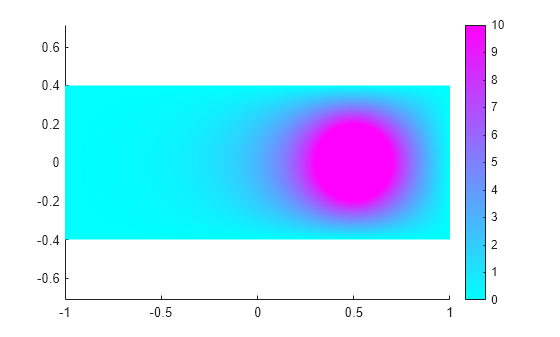
The applyBoundaryCondition function does not set boundary conditions on the edges forming the circle because these are internal edges. To apply boundary conditions on internal edges, use the InternalBC argument.
specifyCoefficients(model,m=0,d=0,c=1,a=0,f=0);
applyBoundaryCondition(model,"dirichlet", ...
                       Edge=1:4,u=0, ...
                       InternalBC=true);
applyBoundaryCondition(model,"dirichlet", ...
                       Edge=5:8,u=10, ...
                       InternalBC=true);
generateMesh(model);
R = solvepde(model);
pdeplot(model,XYData=R.NodalSolution)
axis equal
Input Arguments
Name-Value Arguments
Output Arguments
Tips
When there are multiple boundary condition assignments to the same geometric region, the toolbox uses the last applied setting.
To avoid assigning boundary conditions to a wrong region, ensure that you are using the correct geometric region IDs by plotting and visually inspecting the geometry.
If you do not specify a boundary condition for an edge or face, the default is the Neumann boundary condition with the zero values for
"g"and"q".