step
System object: phased.BackscatterSonarTarget
Namespace: phased
Backscatter incoming sonar signal
Description
Note
Instead of using the step method to perform
the operation defined by the System object™, you can call the object
with arguments, as if it were a function. For example, y
= step(obj,x) and y = obj(x) perform
equivalent operations.
refl_sig = step(target,sig,ang,update)update to
control whether to update the target strength (TS) values. This syntax
applies when you set the Model property to one
of the fluctuating TS models: 'Swerling1', 'Swerling2', 'Swerling3',
or 'Swerling4'. If update is true,
a new TS value is generated. If update is false,
the previous TS value is used.
Note
The object performs an initialization the first time the object is executed. This
initialization locks nontunable properties
and input specifications, such as dimensions, complexity, and data type of the input data.
If you change a nontunable property or an input specification, the System object issues an error. To change nontunable properties or inputs, you must first
call the release method to unlock the object.
Input Arguments
Output Arguments
Examples
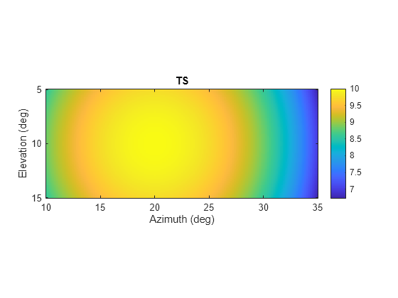
Calculate the reflected sonar signal from a nonfluctuating point target with a peak target strength (TS) of 10.0 db. For illustrative purposes, use a simplified expression for the TS pattern of a target. Real TS patterns are more complicated. The TS pattern covers a range of angles from 10° to 30° in azimuth and from 5° to 15° in elevation. The TS peaks at 20° azimuth and 10° elevation. Assume that the sonar operating frequency is 10 kHz and that the signal is a sinusoid at 9500 kHz.
Create and plot the TS pattern.
azmax = 20.0;
elmax = 10.0;
azpatangs = [10.0:0.1:35.0];
elpatangs = [5.0:0.1:15.0];
tspattern = 10.0*cosd(4*(elpatangs - elmax))'*cosd(4*(azpatangs - azmax));
tspatterndb = 10*log10(tspattern);
imagesc(azpatangs,elpatangs,tspatterndb)
colorbar
axis image
axis tight
title("TS")
xlabel("Azimuth (deg)")
ylabel("Elevation (deg)")
Generate and plot 50 samples of the sonar signal.
freq = 9.5e3;
fs = 100*freq;
nsamp = 500;
t = [0:(nsamp-1)]'/fs;
sig = sin(2*pi*freq*t);
plot(t*1e6,sig)
xlabel("Time (\mu seconds)")
ylabel("Signal Amplitude")
grid

Create the phased.BackscatterSonarTarget System object™.
target = phased.BackscatterSonarTarget(Model="Nonfluctuating", ...
    AzimuthAngles=azpatangs,ElevationAngles=elpatangs, ...
    TSPattern=tspattern);
For a sequence of different azimuth incident angles (at constant elevation angle), plot the maximum scattered signal amplitude.
az0 = 13.0;
el = 10.0;
naz = 20;
az = az0 + [0:1:20];
naz = length(az);
ss = zeros(1,naz);
for k = 1:naz
    y = target(sig,[az(k);el]);
    ss(k) = max(abs(y));
end
plot(az,ss,'o')
xlabel('Azimuth (deg)')
ylabel('Backscattered Signal Amplitude')
grid

Calculate the reflected sonar signal from a Swerling2 fluctuating point target with a peak target strength (TS) of 10.0 db. For illustrative purposes, use a simplified expression for the TS pattern of a target. Real TS patterns are more complicated. The TS pattern covers a range of angles from 10°to 30° in azimuth and from 5° to 15° in elevation. The TS peaks at 20° azimuth and 10° elevation. Assume that the sonar operating frequency is 10 kHz and that the signal is a sinusoid at 9500 kHz.
Create and plot the TS pattern.
azmax = 20.0;
elmax = 10.0;
azpatangs = [10.0:0.1:35.0];
elpatangs = [5.0:0.1:15.0];
tspattern = 10.0*cosd(4*(elpatangs - elmax))'*cosd(4*(azpatangs - azmax));
tspatterndb = 10*log10(tspattern);
imagesc(azpatangs,elpatangs,tspatterndb)
colorbar
axis image
axis tight
title("TS")
xlabel("Azimuth (deg)")
ylabel("Elevation (deg)")

Generate the sonar signal.
freq = 9.5e3;
fs = 10*freq;
nsamp = 50;
t = [0:(nsamp-1)]'/fs;
sig = sin(2*pi*freq*t);
Create the phased.BackscatterSonarTarget System object™.
target = phased.BackscatterSonarTarget(Model="Nonfluctuating", ...
    AzimuthAngles=azpatangs,ElevationAngles=elpatangs, ...
    TSPattern=tspattern,Model="Swerling2");
Compute and plot the fluctuating signal amplitude for 20 time steps.
az = 20.0;
el = 10.0;
nsteps = 20;
ss = zeros(1,nsteps);
for k = 1:nsteps
    y = target(sig,[az;el],true);
    ss(k) = max(abs(y));
end
plot([0:(nsteps-1)]*1000/fs,ss,'o')
xlabel("Time (msec)")
ylabel("Backscattered Signal Amplitude")
grid

Version History
Introduced in R2017a