Modeling Transmitter and Receiver with Increasing Levels of Fidelity
The phased.Transmitter and phased.Receiver System objects can be used to model hardware effects prior to radiation from an antenna array (in the case of phased.Transmitter) or after collection by an antenna array (in the case of phased.Receiver). These objects are used in the Phased Array System Toolbox™ signal propagation workflow and are also used in related Radar Toolbox™ objects such as the radarTransceiver (Radar Toolbox), and bistaticTransmitter (Radar Toolbox) and bistaticReceiver (Radar Toolbox).
These objects provide separate configurations to enable varying levels of model fidelity. This page discusses the conceptual meaning of each configuration of these objects and lays out how they can be used to model signal propagation in a system containing antennas and antenna arrays.
Configurations of Transmitter and Receiver
Effective Isotropic Radiated Power (EIRP) Configuration
The lowest fidelity model, which exists only in the phased.Transmitter System object, can be used to easily model the combined output power due to the effect of a transmit amplifier and antenna without needing to specify any information about saturation effects or antenna patterns.
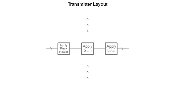
In the "EIRP" configuration, the conceptual model that the transmitter represents is a noiseless linear amplifier which has an output power specified by the PeakPower property and an antenna element which has an antenna gain specified by the Gain property. Additionally, some overall transmission loss can be included as a LossFactor. We can represent such a system visually:
![]()
We can use the viewLayout object function to visualize the order in which effects are applied in the "EIRP" configuration of the phased.Transmitter.
transmitter = phased.Transmitter( ...
    Configuration="EIRP");
figure;
viewLayout(transmitter);
In this configuration of the object, the PeakPower property is only a scaling factor, and is set assuming that the magnitude of the input signal is unity. So, if the magnitude of the input signal is not unity, the output power will not match your expectations. The command line display shows which properties are active in the 'EIRP' configuration:
disp(transmitter);
  phased.Transmitter with properties:

   Configuration
         Configuration: 'EIRP'
       InUseOutputPort: false
    CoherentOnTransmit: true

   Model
             PeakPower: 5000
                  Gain: 20
            LossFactor: 0
Budget Configuration
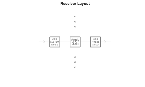
The next level of fidelity is the Budget configuration. This configuration exists in both the phased.Transmitter and phased.Receiver System objects. In this configuration, we model the transmitter or receiver as a summary of effects of all individual components which define the overall dynamic range of the system.
In this configuration of the object we can think of the transmitter or receiver as being modeled as a nonlinear amplifier or a number of parallel amplifiers on each channel. In its simplest form, the amplifier model is linear, but can have nonlinear characteristics as well:
![]()
This configuration allows you to specify noise (which defines the lower end of the dynamic range), a non-linear gain model (which defines the upper end of the dynamic range), and some phase offset difference between each channel. The order in which these effects are applied can be visualized using the viewLayout object function of the phased.Receiver.
receiver = phased.Receiver( ...
    Configuration="Budget");
figure;
viewLayout(receiver);
Because this configuration of the objects maps directly to the Budget, we can model an array of components in the RF Budget Analyzer (RF Toolbox) and export a phased.Transmitter or phased.Receiver in the "Budget" configuration from this app. The command line display shows which properties are active in the 'Budget' configuration:
disp(receiver);
  phased.Receiver with properties:

   Configuration
           Configuration: 'Budget'
         EnableInputPort: false
              SampleRate: 1000000

   Model
              GainMethod: 'Linear'
                    Gain: 20
             NoiseMethod: 'Noise figure'
             NoiseFigure: 3
    ReferenceTemperature: 290
             PhaseOffset: 0

   Input Noise
           AddInputNoise: false

   Randomization
              SeedSource: 'Auto'
Cascade Configuration
The highest level of fidelity is the "Cascade" configuration. This configuration exists in both the phased.Transmitter and phased.Receiver. In this configuration of the object, we model the transmitter or receiver as a cascade of individual hardware components or effects which each affect the signal in series.
In this configuration of the object we can think of the transmitter or receiver as being modeled as a series of components that you can define and customize:
![]()
A list of compatible objects to be used in the "Cascade" configuration of the phased.Transmitter and phased.Receiver can be found at their respective documentation pages.
A simple model of a phased.Transmitter can be created which has only a single linear amplifier in the cascade. We can once again use viewLayout to visualize the order in which effects are applied.
amp = rf.Amplifier(Gain=20);
transmitter = phased.Transmitter(Configuration="Cascade",Cascade={amp});
figure;
viewLayout(transmitter);
The command line display shows which properties are active in the 'Cascade' configuration:
disp(transmitter);
  phased.Transmitter with properties:

   Configuration
      Configuration: 'Cascade'
    InUseOutputPort: false

   Model
            Cascade: {[1×1 rf.Amplifier]}
Example 1: Modeling Transmitted Signal Power and Distortion
In this section, we discuss how we can use the phased.Transmitter in each of the three configurations along with a phased.Radiator System object to preserve the overall power level behavior of the model while introducing new effects at each level of fidelity that might be of interest depending on your requirements.
System and Waveform Definition
The radiating system that we are modeling in this case is a radiator with an antenna array made up of four cosine antenna elements. The peak power out of the transmitter power amplifier (PA) is 100 W, and the antenna gain is defined by the antenna element pattern and geometry.
% Define some high level system parameters
fc = 2.4e9;
fs=1e6;
bw = 1e5;

% Create antenna array model
nElements = 4;
element = phased.CosineAntennaElement;
ula = phased.ULA(Element=element, ...
    NumElements=nElements, ...
    ElementSpacing=freq2wavelen(fc)/2);

% Define output power and antenna gain
pOut = 100;
antennaGain = directivity(ula,fc,[0;0]);
disp(['Max antenna gain is ',num2str(antennaGain)]);
Max antenna gain is 13.1714
We will investigate modeling the transmission of two kinds of waveforms. We look at transmitting a radar waveform to verify that the radiated power matches our expectations at each level of fidelity. We also look at transmitting a communications waveform to investigate the distortions that occur to the radiated waveform according to our transmitter model.
% Create the radar waveform
waveform = phased.LinearFMWaveform(SampleRate=fs,SweepBandwidth=bw);
lfmSig = waveform();

% Create the comms waveform - 16 QAM
M = 16;
nSamples = 100;
refConst = qammod(0:M-1,M,UnitAveragePower=true);
data = randi([0 M-1],nSamples,1);
commSig = qammod(data,M,UnitAveragePower=true);
Transmitter in EIRP Configuration to Model PA Output and Antenna Gain
Let's say we want to easily model a radiated signal out of the transmit antenna at the expected power without considering any directional effects of the antenna or distortions to the transmit waveform. This is the lowest level of fidelity model, but it is very easy to set up using the phased.Transmitter in the "EIRP" configuration.
To do this, set the PeakPower property to represent the power output of the PA and the Gain property to represent the gain of the antenna array. When using using this configuration, if we set the antenna gain in the phased.Transmitter, we must use a phased.IsotropicAntennaElement instead of an array with directional gain as our radiating element so as not to double count antenna gain.
Create the transmitter object.
transmitter = phased.Transmitter(Configuration="EIRP", ...
    PeakPower=pOut,Gain=antennaGain);
Create an antenna model with an Isotropic Antenna Element.
antenna = phased.Radiator(Sensor=phased.IsotropicAntennaElement(),OperatingFrequency=fc);
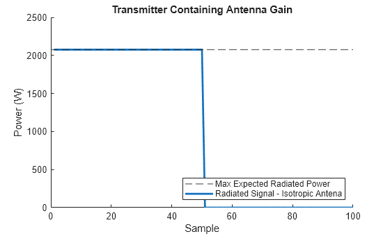
Propagate the signal, radiating to boresight.
radAngle = [0;0];
txSig = transmitter(lfmSig);
radSig = antenna(txSig,radAngle);
We expect the output signal to have a power of 100W amplified by antenna gain.
maxExpectedPower = pOut*db2pow(antennaGain);
plotSignalPower(radSig, ...
    'Radiated Signal - Isotropic Antena',maxExpectedPower, ...
    'Max Expected Radiated Power', ...
    'Transmitter Containing Antenna Gain');
In this configuration, we do not see any directional effects due to the antenna pattern, assuming that the antenna gain is uniform in all directions. To demonstrate this, we can look at what happens when we radiate in a direction other than boresight.
Propagate the signal, radiating off-boresight:
radAngle = [45;0];
txSig = transmitter(lfmSig);
radSig = antenna(txSig,radAngle);
Off-boresight radiation still has maximum power in this simplified model.
maxExpectedPower = pOut*db2pow(antennaGain);
plotSignalPower(radSig, ...
    'Radiated Signal - Off Boresight', ...
    maxExpectedPower,'Max Expected Radiated Power', ...
    'Transmitter Containing Antenna Gain - Off Boresight');
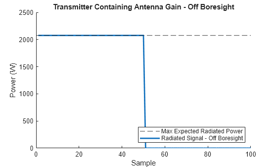
We can see that using this model, no directional effects are captured.
Furthermore, we can demonstrate that no signal distortions are present using this model by radiating the communciations signal.
Radiate the communications signal.
radAngle = [0;0];
txSig = transmitter(commSig);
radSig = antenna(txSig,radAngle);
Show constellation diagram.
showConstellationDiagram(radSig,refConst)
![]()
No distortions to the transmitted waveform are apparent at this level of fidelity.
Transmitter in EIRP Configuration to Model PA Output with Separate Antenna Model
To enhance the modeling fidelity, instead of using a single radiating element and allocating all antenna gain to the Gain property of the phased.Transmitter by using a single phased.IsotropicAntennaElement, we can include a model of our antenna array.
Create an antenna model using a ULA.
antenna = phased.Radiator(Sensor=ula, ...
    SensorGainMeasure="dBi", ...
    OperatingFrequency=fc);
We once again use the phased.Transmitter in the "EIRP" configuration, however because we are using a model of our antenna with directional gain, we set the Gain property in the phased.Transmitter to zero so as not to double count antenna gain.
Create the transmitter.
transmitter = phased.Transmitter(Configuration="EIRP",PeakPower=pOut,Gain=0);
Propagate the signal, radiating to boresight.
radAngle = [0;0];
txSig = transmitter(lfmSig);
radSig = antenna(txSig,radAngle);
We expect the output signal to have a power of 100W amplified by the antenna gain.
plotSignalPower(radSig,'Radiated Signal - With Antenna Model',maxExpectedPower,'Expected Radiated Power','Transmitter with Antenna Model');
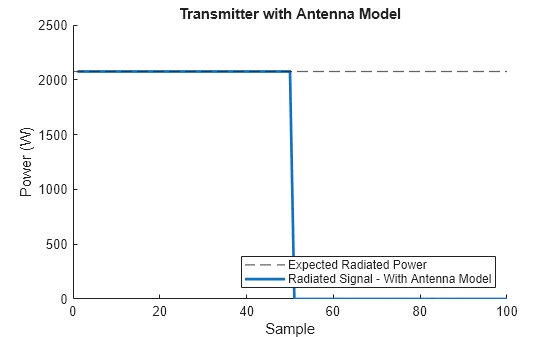
The power in this case still matches our expectations. The model including the antenna gain is marginally more difficult to set up and may be less performant, but we can now model directional gain. For example, if we radiate to a non-boresight direction, radiated signal power should be reduced.
Propagate the signal, radiating off-boresight.
radAngle = [15;0];
txSig = transmitter(lfmSig);
radSig = antenna(txSig,radAngle);
We expect the signal power to be reduced when propagating off-boresight direction due to the inclusion of the antenna model.
plotSignalPower(radSig,"Radiated Signal - Off Boresight", ...
    maxExpectedPower,"Radiated Power - Boresight", ...
    "Transmitter with Antenna Model - Off Boresight");
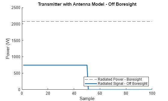
We can see that the power radiated off-boresight is lower using this model, as we would expect.
Although we can now model directional effects, still no signal distortions are present because we are using the "EIRP" configuration which only applies simple scaling factors to the signal. We can again demonstrate this by radiating the communications signal and visualizing the constellation diagram.
Radiate the communications signal.
radAngle = [0;0];
txSig = transmitter(commSig);
radSig = antenna(txSig,radAngle);
Show constellation diagram
showConstellationDiagram(radSig,refConst)
![]()
No distortions to the transmitted waveform are apparent at this level of fidelity.
Transmitter in Budget Configuration to Model Saturation
If we want to capture non-linear effects of the PA in our transmitter, the "EIRP" configuration does not suffice. We can use the "Budget" configuration to model a transmitter operating in saturation.
In this discussion we define non-linear amplification using a cubic polynomial model which requires users to specify linear gain (using the Gain property) and the output third-order intercept point (OIP3), which is a common measure of system nonlinearity. A linear gain of 50 dB and OIP3 of 58.3 corresponds to a saturation output power of about 100W, which is the output power of our previously defined transmitter. Nonlinearities and Noise in Idealized Baseband Amplifier Block (RF Blockset) is a good reference for relating OIP3 to output saturation power.
We set up a phased.Transmitter below to recreate the system shown in the "EIRP" section while modeling transmitter saturation and visualize the input power to output power relationship using the viewGain method.
Define a transmitter with a nonlinearity.
transmitter = phased.Transmitter(Configuration="Budget",GainMethod="Cubic polynomial",...
    Gain=50,OIP3=58.3);
figure
viewGain(transmitter)
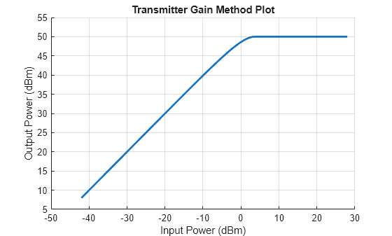
This plot shows that the transmitter saturates at an input power at about 0 dBm (0.01 W) and the saturation output power is 50 dBm (100W). So our input signal at 1W will be output at 100W.
Reusing the antenna defined in the section above, we can see that the total radiated power using this model is unchanged. This meets our expectations.
% Propagate the signal with nonlinear amplifier, radiating to boresight
radAngle = [0;0];
release(antenna);
txSig = transmitter(lfmSig);
radSig = antenna(txSig,radAngle);
We expect the signal power to be the same as the max expected power from above.
plotSignalPower(radSig,"Radiated Signal - Nonlinear Transmitter", ...
    maxExpectedPower,"Expected Radiated Power", ...
    "Transmitter with Nonlinear Amplification");
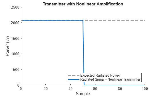
In addition to correctly modeling the output power of our uniform amplitude radar waveform, this model also will capture waveform distortions that were not being captured using the lower level of fidelity. This distortion is apparent when transmitting the communications waveform near the saturation point of our system.
To demonstrate this distortion, we scale the communications waveform so it is just below the saturation level of the transmitter, and visualize the constellation diagram of the radiated waveform.
Scale signal so that it is below the saturation level of the transmitter.
pSatdBm = 5;
pSigMaxdBm = pSatdBm-5;
pSigMaxMag = db2mag(pSigMaxdBm-30);
commSigIn = commSig/max(abs(commSig))*pSigMaxMag;
Pass the signal through the transmitter and then radiate the signal.
radAngle = [0;0];
txSig = transmitter(commSigIn);
radSig = antenna(txSig,radAngle);
View the constellation diagram.
showConstellationDiagram(radSig,refConst)
![]()
We can see that when the signal is transmitted near the saturation level of the receiver, the signal gets distorted. By using a transmitter model with non-linear gain in the "Budget" configuration, we see signal distortions that would not be apparent in the "EIRP" configuration of this object.
Transmitter in Cascade Configuration to Model Saturation with Phase Noise
Although the "Budget" configuration of the phased.Transmitter enables some additional impairment modeling, it is limiting in the effects that are available and the order in which those effects are applied. If we want to model additional effects of a transmitter chain, we can use the "Cascade" configuration.
In this section, we develop a higher fidelity model of the phased.Transmitter from above by using an rf.Amplifier (RF Toolbox) to model the PA that is primarily responsible for the saturation effects of the system while also including an rf.Mixer (RF Toolbox) to model phase noise that would be present in the signal due to mixing our baseband signal with a local oscillator.
Create the transmitted signal.
waveform = phased.LinearFMWaveform(SampleRate=fs,SweepBandwidth=bw);
lfmSig = waveform();
Create a mixer to add phase noise to the signal.
mixer = rf.Mixer(IncludePhaseNoise=true, ...
    PhaseNoiseFrequencyOffset=[2000 20000], ...
    PhaseNoiseLevel=[-80 -90], ...
    SampleRate=waveform.SampleRate);
Create an amplifier with the same amplification model as in the "Budget" configuration.
pa = rf.Amplifier(Model='cubic', ...
    Gain=50,OIP3=58.3);
We can combine the effects of our mixer and amplifier in series by using the phased.Transmitter in the "Cascade" configuration. We can visualize the layout using viewLayout to ensure that it matches our expectations.
transmitter = phased.Transmitter(Configuration="Cascade",Cascade={mixer,pa});
figure;
viewLayout(transmitter)
With the model created, we can verify that the output power of the radiated signal matches the output power of the radiated signal when using the lower fidelity "Budget" and "EIRP" models. We expect the final output power to be the same because of the configuration of the power amplifier in the transmitter cascade.
Propagate the signal with nonlinear amplifier, radiating to boresight.
radAngle = [0;0];
release(antenna);
txSig = transmitter(lfmSig);
radSig = antenna(txSig,radAngle);
We expect the signal power to be the same as before.
plotSignalPower(radSig, ...
    'Radiated Signal - Cascade Transmitter', ...
    maxExpectedPower, ...
    'Expected Radiated Power', ...
    'Transmitter Cascade with Mixer and Power Amplifier');
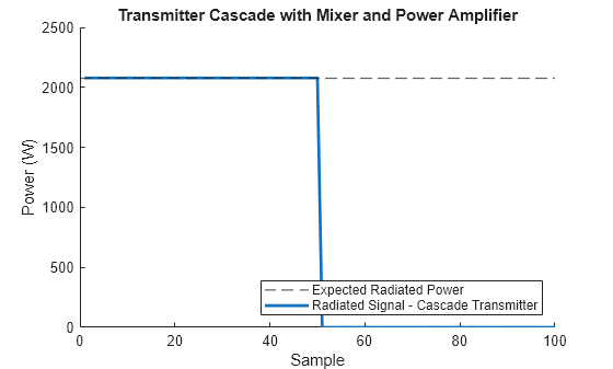
This model matches the lower fidelity models in terms of gross output power, but in this case we have also applied the phase noise that is added by the mixer. We can most easily visualize this additional impairment by once again plotting the constellation diagram of a transmitted communications signal.
Pass the signal through the transmitter and radiate the signal.
radAngle = [0;0];
release(antenna);
txSig = transmitter(commSigIn);
radSig = antenna(txSig,radAngle);
View constellation diagram.
showConstellationDiagram(radSig,refConst)
![]()
Similarly to the constellation diagram in the "Budget" section, we see that some distortion has occured due to the non-linear amplification in the transmitter. However, in this case we also see the additional effects of the mixer phase noise in the variance of the phase at each constellation point.
Example 2: Modeling Receiver Dynamic Range and Interference Effects
In this section, we look at how to model a receiver dynamic range at increasing levels of fidelity using the phased.Receiver in the "Budget" and "Cascade" configurations. Also, we model the effects of a high power interferer on the received signal to see how this model changes with additional considerations such as a passband filter.
System and Waveform Definition
The receiver that we are modeling in this section has a noise floor that is determined by the noise figure of the system and some saturation power level. We define some high level operating parameters here, including a lookup table that defines the receiver gain characteristics.
Define receiver noise characteristics.
nf = 15;
refTemp = 290;
fs = 40e6;
Define carrier frequency.
fc = 1e9;
The linear gain is 30 dB the and saturation input power is 50 dBm.
linGain = 30;
satPowIn = 50;
lookupTable = [-120 -120+linGain 0;
       satPowIn satPowIn+linGain 0;
       satPowIn+30 satPowIn+linGain 0];
The waveform of interest in this case will once again be a radar waveform, but we will also add to this a high power single tone interferer to see how the received signal is impacted.
Create LFM at 0 dBm.
bw = 1e6;
pulseWidth = 500/fs;
prf = 1/(10*pulseWidth);
lfmPowDbm = 0;
lfmAmp = db2mag(0-30);
lfm = phased.LinearFMWaveform(SampleRate=fs,PulseWidth=pulseWidth,PRF=prf,SweepBandwidth=bw,SweepInterval="Symmetric");
lfmSig = lfmAmp*lfm();
Create an interfering tone at the saturation level of the receiver.
interfererAmp = db2mag(satPowIn-30);
fi = 7.5e6;
nSamples = (1/prf)*fs;
interferer = dsp.SineWave(Amplitude=interfererAmp, ...
    Frequency=fi,ComplexOutput=true, ...
    SampleRate=fs,SamplesPerFrame=nSamples);
Combine signal and interferer and visualize the spectrum.
sigWithInt = lfmSig + interferer();
figure;
pspectrum(sigWithInt)
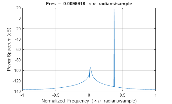
We can see the signal of interest near the center of the spectrum and the high power interfering tone.
Receiver in Budget Configuration to Model Dynamic Range and Interference Effects
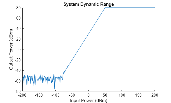
We can define a phased.Receiver in the "Budget" configuration, specifying a noise figure and gain profile to define the overall dynamic range of the system. The dynamic range is defined by the noise floor at the low end and the saturation level at the high end.
receiver = phased.Receiver(Configuration="Budget", ...
    SampleRate=fs,GainMethod='Lookup table', ...
    Table=lookupTable,NoiseMethod="Noise figure", ...
    NoiseFigure=nf, ...
    ReferenceTemperature=refTemp);
Plot the receiver dynamic range.
plotDynamicRange(receiver);
To demonstrate how we might use such a receiver model, we can look at how the presence of the interfering signals near the saturation level of the receiver can distort the spectrum of the desired signal.
To do so, we propagate the signal with the high power interferer created in the previous section through the receiver.
figure;
rxSig = receiver(sigWithInt);
pspectrum(rxSig);
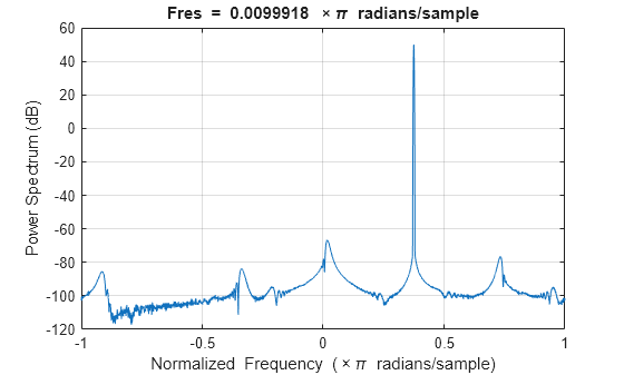
We see substantial distortion in the power spectrum of the received signal due to intermodulation with the interferer near the saturation level of the receiver.
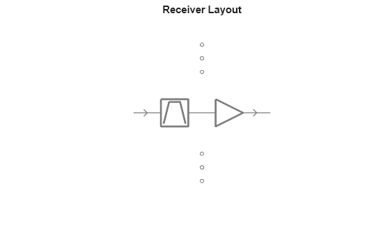
Receiver in Cascade Configuration to Model Dynamic Range and Interference Effects with Filter
In reality, our system may have a bandpass filter to filter out noise and interference outside of our band of interest. It is possible to configure the phased.Receiver to include a filter in the "Cascade" configuration to demonstrate the impact that such a filter has on the distortion of the frequency spectrum of the received signal with the high power interferer.
In this section we define a receiver that has a similar dynamic range to the one discussed in the previous section, characterized by the low noise amplifier (LNA). However, in this case we use the configuration to also place a passband filter at the beginning of the receiver to mitigate the issues with a high power interferer that were demonstrated previously.
We use an rf.Amplifier to represent the LNA and an rf.Filter (RF Toolbox) to filter out signals outside of the bandwidth of the sensing waveform to avoid the effects of the high power interferer.
Create a passband filter.
filtBand = [fc-bw fc+bw];
filter = rf.Filter(ResponseType='bandpass', ...
    PassFreq_bp=filtBand,SampleRate=fs, ...
    RF=fc);
Create the LNA.
lna = rf.Amplifier(Model='ampm',Table=lookupTable,IncludeNoise=true,NF=nf,SampleRate=fs);Create and visualize the receiver.
receiver = phased.Receiver(Configuration="Cascade", ...
    Cascade={filter,lna});
figure;
viewLayout(receiver);
Visualize receiver dynamic range.
plotDynamicRange(receiver);

The dynamic range of the system is relatively unchanged when modeling using a filter and amplifier versus using the lower fidelity "Budget" configuration.
Using this model, we can examine the effects of the high power interferer once again using a plot of the power spectrum.
rxSig = receiver(sigWithInt);
figure;
pspectrum(rxSig);
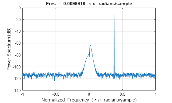
In this case, when we propagate the signal with the high power interferer, the distortion in the frequency spectrum is substantially reduced because of the presence of the bandpass filter.
Multi-Channel Modeling
EIRP Multi-Channel Modeling - Broken PA
You can also model multi-channel behavior in using the "EIRP" configuration of the phased.Transmitter. The number of channels to model can be defined in two ways:
By using a multi-channel (multi-column) input.
By configuring the object with multi-channel behavior.
Some of the properties in the "EIRP" configuration of the phased.Transmitter can be set so that the behavior between channels is different. If you do not configure the object this way but provide a multi-channel input, the behavior between channels will be the same.
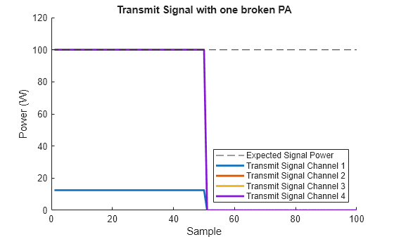
For example, say you want to model a transmitter with four PAs, but one is broken and producing less powerful output. You could configure the object to model this and see what is the impact on the transmitted signal.
Create the waveform.
lfm = phased.LinearFMWaveform(SampleRate=1e6,SweepBandwidth=1e5);
lfmSig = lfm();
Create the transmitter.
pOutMultiChannel = [pOut/8 pOut pOut pOut];
transmitter = phased.Transmitter(Configuration="EIRP", ...
    PeakPower=pOutMultiChannel,Gain=0);
Propagate the input signal and visualize the multi-channel output.
txSig = transmitter(lfmSig);
plotSignalPower(txSig, ...
    'Transmit Signal Channel',pOut, ...
    'Expected Signal Power', ...
    'Transmit Signal with one broken PA');
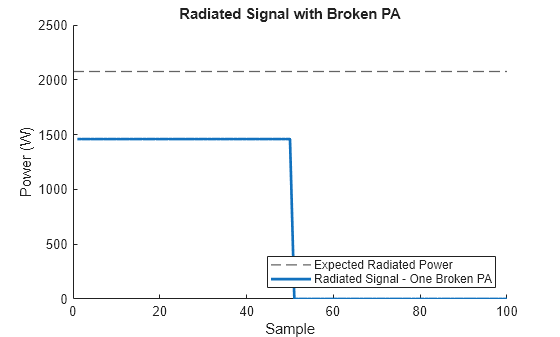
We can then take the output of the transmtter and radiate it through the antenna to see the overall impact on transmit power.
Propagate the signal, radiating to boresight.
radAngle = [0;0];
release(antenna);
radSig = antenna(txSig,radAngle);
We expect the signal power to be reduced when propagating to an off-boresight direction due to the inclusion of the antenna model.
plotSignalPower(radSig, ...
    'Radiated Signal - One Broken PA',maxExpectedPower, ...
    'Expected Radiated Power', ...
    'Radiated Signal with Broken PA');
Budget Multi-Channel Modeling - Calibration Errors
Multi-channel modeling is available in the "Budget" configuration similarly to the "EIRP" configuration. The number of channels to model can be defined in two ways:
By using a multi-channel (multi-column) input.
By configuring the object with multi-channel behavior.
Some of the properties in the "Budget" configuration of the phased.Transmitter and phased.Receiver can be set so that the behavior between channels is different. If you do not configure the object this way but provide a multi-channel input, the behavior between channels will be the same.
See Hardware Array Data Collection and Simulation for an example regarding how you can use differential phase offsets between the channels in a receiver to model calibration errors encountered in a real system.
Cascade Multi-Channel Modeling - Hybrid Impairment Modeling
Multi-channel modeling is available in the "Casade" configuration similarly to the "EIRP" and "Budget" configurations. The number of channels to model can be defined in two ways:
By using a multi-channel (multi-column) input.
By configuring the cascade with multi-channel objects.
If the cascade is defined with only single channel objects, then if a multi-channel input is given the single channel objects are expanded to multiple channels operating in parallel.
See Modeling Impairments in Phased Arrays with Hybrid Architectures for an example on defining multi-channel behavior using an analog beamformer model or Create a Digital Twin of a TI mmWave Radar (Radar Toolbox) for an example that simulates a real radar using time division multiplexing.
Helper Functions
function plotSignalPower(sig,sigName,expectedPower,expectedPowerName,t)
    ax = axes(figure);
    hold(ax,"on");
    xlabel(ax,"Sample");
    ylabel(ax,"Power (W)");
    yline(ax,expectedPower,DisplayName=expectedPowerName,LineStyle='--',LineWidth=1);

    nChannel = size(sig,2);
    if nChannel == 1
        plot(ax,abs(sig).^2,DisplayName=sigName,LineWidth=2);
    else
        for iSig = 1:nChannel
            plot(ax,abs(sig(:,iSig)).^2,DisplayName=[sigName,' ',num2str(iSig)],LineWidth=2);
        end
    end

    title(ax,t);
    legend(ax,Location="southeast");
end

function plotDynamicRange(sys)
    % Input a large signal range and plot output to visualize dynamic range
    inPowDbm = (-200:200);
    inSig = db2mag(inPowDbm-30);
    out = sys(inSig);
    outPowDbm = mag2db(abs(out))+30;
    ax = axes(figure);
    hold(ax,"on");
    plot(ax,inPowDbm,outPowDbm);
    title(ax,"System Dynamic Range");
    xlabel(ax,"Input Power (dBm)");
    ylabel(ax,"Output Power (dBm)");
    release(sys);
end

function showConstellationDiagram(inSig,refConst)
    const = comm.ConstellationDiagram(ReferenceConstellation=refConst);
    inputScaled = inSig/max(abs(inSig))*max(abs(refConst));
    const(inputScaled);
end
See Also
phased.Receiver | phased.Transmitter | rf.Amplifier (RF Toolbox) | rf.Mixer (RF Toolbox) | rf.PAmemory (RF Toolbox) | rf.Sparameter (RF Toolbox) | rf.Sparameter (RF Toolbox) | radarbudgetplot (Radar Toolbox)