Imitate Nonlinear MPC Controller for Sliding Robot
This example shows how to train, validate, and test a deep neural network (DNN) that imitates the behavior of a nonlinear model predictive controller for a robot sliding over a 2-D frictionless plane, modeled in Simulink®. It then compares the behavior of the deep neural network with that of the original controller. To train the deep neural network, this example uses the data aggregation (DAgger) approach described in [1].
Nonlinear model predictive control (NLMPC) solves a constrained nonlinear optimization problem in real time based on the current state of the plant. For more information on NLMPC, see Nonlinear MPC (Model Predictive Control Toolbox). For an example that uses two nonlinear MPC controllers to respectively generate and track an optimal trajectory for a sliding robot model, see Trajectory Optimization and Control of Sliding Robot Using Nonlinear MPC (Model Predictive Control Toolbox). For an example that instead uses a reinforcement learning agent to solve the control problem for a sliding robot, see Train DDPG Agent to Control Two-Thruster Sliding Vehicle.
Replacing an NLMPC controller with a trained DNN can be an appealing option because evaluating a DNN can be more computationally efficient than solving a nonlinear optimization problem in real-time. For an example that replaces a classical MPC controller with a neural network, see Imitate MPC Controller for Lane Keeping Assist.
If the trained DNN reasonably approximates the controller behavior, you can then deploy the network for your control application. You can also use the network as a warm starting point for training the actor network of a reinforcement learning agent. For an example that does so with a DNN trained for an MPC application, see Train DDPG Agent with Pretrained Actor Network.
Design Nonlinear MPC Controller
Design a nonlinear MPC controller for a sliding robot. The dynamics for the sliding robot are the same as in Trajectory Optimization and Control of Sliding Robot Using Nonlinear MPC (Model Predictive Control Toolbox) example, and are described in [2]. First, define the limit for the control variables, which are the robot thrust levels.
umax = 3;
Create the nonlinear MPC controller object nlobj. To reduce command-window output, disable the MPC update messages. For more information, see nlmpc (Model Predictive Control Toolbox).
mpcverbosity off;
nlobj = createMPCobjImSlidingRobot(umax);
Prepare Input Data
Load the input data from DAggerInputDataFileImSlidingRobot.mat. The columns of the data set contain:
is the position of the robot along the x-axis.
is the position of the robot along the y-axis.
is the orientation of the robot.
is the velocity of the robot along the x-axis.
is the velocity of the robot along the y-axis.
is the angular velocity of the robot.
is the thrust on the left side of the sliding robot
is the thrust on the right side of the sliding robot
is the thrust on the left side computed by NLMPC
is the thrust on the right side computed by NLMPC
The data in DAggerInputDataFileImSlidingRobot.mat is created by computing the NLMPC control action for randomly generated states (, , , , , ), and previous control actions (, ). To generate your own training data, use the collectDataImSlidingRobot function.
Load the input data.
fileName = "DAggerInputDataFileImSlidingRobot.mat";
DAggerData = load(fileName);
data = DAggerData.data;
existingData = data;
numCol = size(data,2);
Create Deep Neural Network
Create the deep neural network that will imitate the NLMPC controller after training. The network architecture uses the following types of layers.
imageInputLayeris the input layer of the neural network.fullyConnectedLayermultiplies the input by a weight matrix and then adds a bias vector.reluLayeris the activation function of the neural network.tanhLayerconstrains the value to the range to [-1,1].scalingLayerscales the value to the range to [-3,3].
Define the network as an array of layer objects.
numObs = numCol-2;
numAct = 2;
hiddenLayerSize = 256;
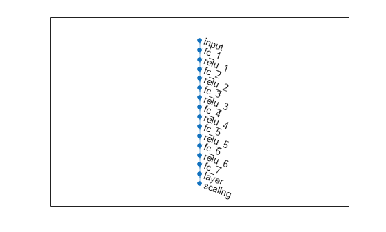
imitateMPCNetwork = [
featureInputLayer(numObs)
fullyConnectedLayer(hiddenLayerSize)
reluLayer
fullyConnectedLayer(hiddenLayerSize)
reluLayer
fullyConnectedLayer(hiddenLayerSize)
reluLayer
fullyConnectedLayer(hiddenLayerSize)
reluLayer
fullyConnectedLayer(hiddenLayerSize)
reluLayer
fullyConnectedLayer(hiddenLayerSize)
reluLayer
fullyConnectedLayer(numAct)
tanhLayer
scalingLayer(Scale=umax)
];
Plot the network.
plot(dlnetwork(imitateMPCNetwork))
Behavior Cloning Approach
One approach to learning an expert policy using supervised learning is the behavior cloning method. This method divides the expert demonstrations (NLMPC control actions in response to observations) into state-action pairs and applies supervised learning to train the network.
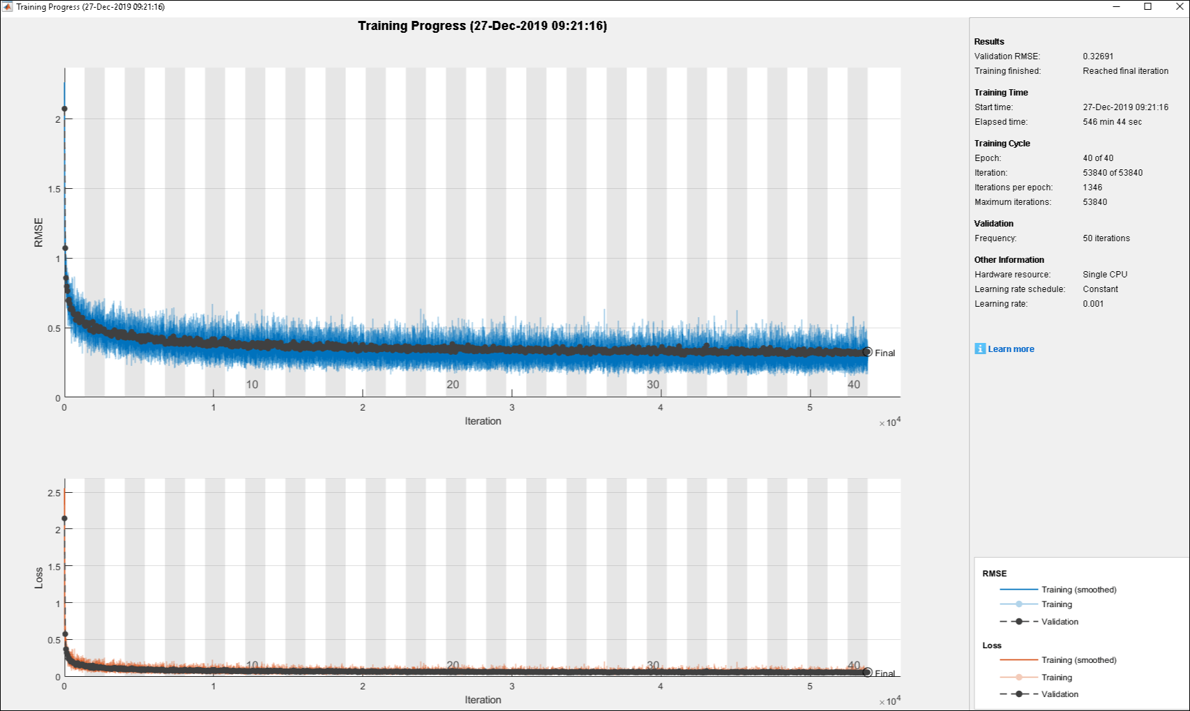
Specify training options.
% Initialize validation cell array
validationCellArray = {0,0};

options = trainingOptions("adam", ...
    Metrics="rmse", ...
    Shuffle="every-epoch", ...
    MiniBatchSize=512, ...
    ValidationData=validationCellArray, ...
    InitialLearnRate=1e-3, ...
    ExecutionEnvironment="cpu", ...
    GradientThreshold=10, ...
    MaxEpochs=40 ...
    );
You can train the behavior cloning neural network by following below steps:
Collect data using the
collectDataImSlidingRobotfunction.Train the behavior cloning network using the
behaviorCloningTrainNetworkfunction.
The training of the DNN using behavior cloning reduces the gap between the DNN and NLMPC performance. However, the behavior cloning neural network fails to imitate the behavior of the NLMPC controller correctly on some randomly generated data.
Training a DNN is a computationally intensive process. For this example, to save time, load a pretrained neural network object.
load("behaviorCloningMPCImDNNObject.mat");Data Aggregation Approach
To improve the performance of the DNN, you can learn the policy using an interactive demonstrator method. DAgger is an iterative method where the DNN is run in the closed-loop environment. The expert, in this case the NLMPC controller, outputs actions based on the states visited by the DNN. In this manner, more training data is aggregated and the DNN is retrained for improved performance. For more information, see [1].
Train the deep neural network using the DAggerTrainNetwork function. It creates DAggerImSlidingRobotDNNObj.mat file that contains the following information.
DatasetPath:path where the dataset corresponding to each iteration is storedpolicyObjs:policies that were trained in each iterationfinalData:total training data collected till final iterationfinalPolicy:best policy among all the collected policies
First, create and initialize the parameters for training. Use the network trained using behavior cloning (behaviorCloningNNObj.imitateMPCNetObj) as the starting point for the DAgger training.
[dataStruct,nlmpcStruct,tuningParamsStruct,neuralNetStruct] = ...
    loadDAggerParameters(existingData,numCol,nlobj,umax, ...
    options, behaviorCloningNNObj.imitateMPCNetObj);
To save time, load a pretrained neural network by setting doTraining to false. To train the DAgger yourself, set doTraining to true.
doTraining = false;

if doTraining
    DAgger = DAggerTrainNetwork( ...
        nlmpcStruct, ...
        dataStruct, ...
        neuralNetStruct, ...
        tuningParamsStruct);
else
    load("DAggerImSlidingRobotDNNObj.mat");
end
DNN = DAgger.finalPolicy;
As an alternative, you can train the neural network with a modified policy update rule using the DAggerModifiedTrainNetwork function. In this function, after every 20 training iterations, the DNN is set to the most optimal configuration from the previous 20 iterations. To run this example with a neural network object with the modified DAgger approach, use the DAggerModifiedImSlidingRobotDNNObj.mat file.
Compare Trained DAgger Network with NLMPC Controller
To compare the performance of the NLMPC controller and the trained DNN, run closed-loop simulations with the sliding robot model.
Set initial condition for the states of the sliding robot (, , , , , ) and the control variables of sliding robot (, ).
x0 = [-1.8200 0.5300 -2.3500 1.1700 -1.0400 0.3100]';
u0 = [-2.1800 -2.6200]';
Define simulation duration, sample time and number of simulation steps.
% Duration
Tf = 15;

% Sample time
Ts = nlobj.Ts;

% Simulation steps
Tsteps = Tf/Ts+1;
Run a closed-loop simulation of the NLMPC controller.
tic
[xHistoryMPC,uHistoryMPC] = ...
    simModelMPCImSlidingRobot(x0,u0,nlobj,Tf);
toc
Elapsed time is 13.823314 seconds.
Run a closed-loop simulation of the trained DAgger network.
tic
[xHistoryDNN,uHistoryDNN] = ...
    simModelDAggerImSlidingRobot(x0,u0,DNN,Ts,Tf);
toc
Elapsed time is 0.948931 seconds.
Plot the results, and compare the NLMPC and trained DNN trajectories.
plotSimResultsImSlidingRobot(nlobj, ...
    xHistoryMPC,uHistoryMPC,xHistoryDNN,uHistoryDNN,umax,Tf);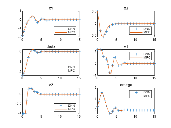
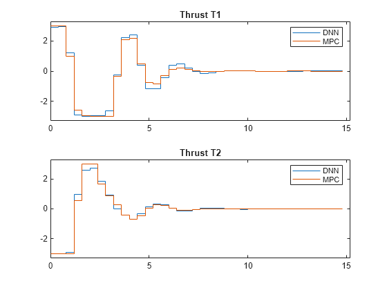
The DAgger neural network successfully imitates the behavior of the NLMPC controller. The sliding robot states and control action trajectories for the controller and the DAgger deep neural network closely align. The closed-loop simulation time for the DNN is significantly less than that of the NLMPC controller.
Animate the Sliding Robot with Trained DAgger Network
To validate the performance of the trained DNN, animate the sliding robot with data from the DNN closed-loop simulation. The sliding robot lands at the origin successfully.
Lx = 5;
Ly = 5;
for ct = 1:Tsteps
    x = xHistoryDNN(ct,1);
    y = xHistoryDNN(ct,2);
    theta = xHistoryDNN(ct,3);
    tL = uHistoryDNN(ct,1);
    tR = uHistoryDNN(ct,2);
    plotSlidingRobot(x,y,theta,tL,tR,Lx,Ly);
    pause(0.05);
end
% Turn on MPC messages
mpcverbosity on;
References
[1] Osa, Takayuki, Joni Pajarinen, Gerhard Neumann, J. Andrew Bagnell, Pieter Abbeel, and Jan Peters. ‘An Algorithmic Perspective on Imitation Learning’. Foundations and Trends in Robotics 7, no. 1–2 (2018): 1–179. https://doi.org/10.1561/2300000053.
[2] Y. Sakawa. "Trajectory planning of a free-flying robot by using the optimal control.", Optimal Control Applications and Methods, Vol. 20, 1999, pp. 235-248.
See Also
Functions
trainNetwork|predict|nlmpcmove(Model Predictive Control Toolbox)
Objects
SeriesNetwork|nlmpc(Model Predictive Control Toolbox)
Topics
- Imitate MPC Controller for Lane Keeping Assist
- Train DDPG Agent to Control Two-Thruster Sliding Vehicle
- Trajectory Optimization and Control of Sliding Robot Using Nonlinear MPC (Model Predictive Control Toolbox)
- Train DDPG Agent with Pretrained Actor Network
- Nonlinear MPC (Model Predictive Control Toolbox)