Tune Fixed PI Gains Using Reinforcement Learning

R2026b

This example shows how to use reinforcement learning (RL) to tune a single, fixed, set of proportional-integral (PI) gains of a PID controller.

Specifically, this example shows the first of three common approaches to using RL for PI parameter tuning. The three approaches are described in Tuning PI Gains Using Reinforcement Learning and are as follows:

1) Single Fixed Gains Across Multiple Operating Points (this example)

2) Fixed Set of Gains per Initial Condition, see Schedule PI Gains Per Initial Condition Using Reinforcement Learning.

3) Online Dynamically Adaptive Gains, see Dynamically Adapt PI Gains Online Using Reinforcement Learning.

With the approach shown in this example, the goal is to find one proportional and one integral gain that perform well across different operating conditions. This approach is adequate in a scenario in which you know that the plant initial and operating conditions do not substantially change or they do not substantially affect the plant behavior. In other words, in this scenario, you expect a single, fixed, PI controller to be able to drive the plant towards the desired behavior, independently on the plant initial condition.

For more information, see Tuning PI Gains Using Reinforcement Learning.

Open Simulink Model

The plant model in this example is a water tank, implemented in the Simulink® model watertankLQG.slx, which is included as a supporting file. The model includes a PI controller that maintains the water level in the tank at a reference value.

Open the model.

WaterTankModel = 'watertankLQG';
open_system(WaterTankModel)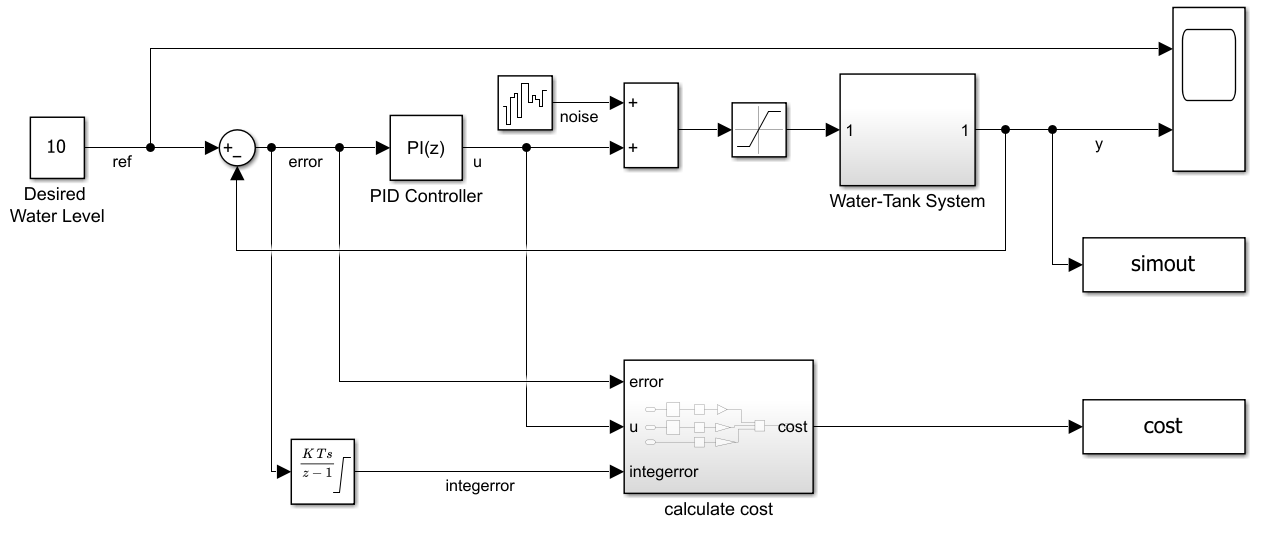

The two To Workspace blocks simout and cost save the water level signal y and the cost signal, respectively, to the MATLAB® workspace, for later inspection. The model includes process noise with variance $E\left(n^2\left(t\right)\right)=0.01$.

The PID controller block used in the model implements a discrete-time PI controller. To maintain the water level $y$ at the target value while minimizing control action u, the PI gains of the PID controller are chosen, using the Control System Tuner (CST), to minimize the cumulative cost. This cumulative cost corresponds to the following linear quadratic Gaussian (LQG) criterion:

$$J_{\text{LQG}}=\underset{T\Rightarrow \infty }{\lim }E\left(\frac{1}{T}\sum _{t=0}^T\left({\left(\text{Href}-y\left(t\right)\right)}^2+0.01u^2\left(t\right)+0.0001{\left(\sum _{k=0}^t\text{Ts}\left(\text{Href}-y\left(k\right)\right)\right)}^2\right)\right)$$

Here, $J_{LQG}$ is the cumulative cost, $\text{Href}$ is the desired water level, T is the number of time steps, and $\text{Ts}$ is the sample time.

The term $\sum _{k=0}^t\text{Ts}\left(\text{Href}-y\left(k\right)\right)$ is the discrete-time integral of the error, which is also calculated inside the PID controller block and fed back as a part of the control signal through the integral gain Ki to keep the steady-state error close to zero. For consistency with the examples that show other approaches, and with the PI controller designed using CST, this example uses $J_{LQG}$ as cost to minimize. For more information on using Control System Tuner, see Tune a Control System Using Control System Tuner (Simulink Control Design).

To simulate the controller in this model, you must specify the simulation time Tf and the controller sample time Ts, in seconds.

Ts = 1;
Tf = 100;

For more information about the water tank model, see watertank Simulink Model (Simulink Control Design).

Specify Random Number Stream Seed and Algorithm for Reproducibility

The example code might involve computation of random numbers at several stages. Fixing the random number stream at the beginning of some sections in the example code preserves the random number sequence in the section every time you run it, which is a necessary condition to reproduce the results. For more information, see Results Reproducibility.

Specify the random number stream with the seed 0 and random number algorithm Mersenne Twister. For more information on controlling the seed used for random number generation, see rng.

previousRngState = rng(0,"twister");

The output previousRngState is a structure that contains information about the previous state of the stream. You will restore the state at the end of the example.

Create Environment Object

In this example, you model the PI controller as a reinforcement learning policy that is linear in the observation, which is the vector containing the error and its integral.

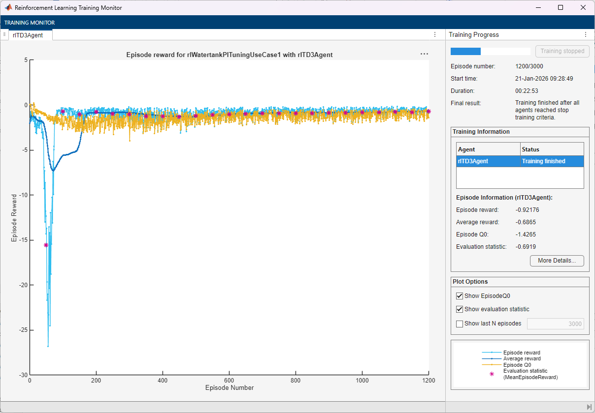
The training session consists of 3000 episodes, where each episode is a simulation of the Simulink closed loop model lasting 100 time steps. During the simulation, the reinforcement learning agent acts on the pump, observes the water level and its corresponding reward, and uses these observations to tune the weights of its actor model (which are the two PI gains) to maximize the expected cumulative reward.

Modify the water tank Simulink model using the following steps.

1. Delete the PID Controller block.

2. Insert an RL Agent block in place of the PID Controller block.

3. Create the observation vector ${\left[\begin{array}{ccc}\int e\text{dt}& e& \end{array}\right]}^T$, where $e=Href-y$, $y$ is the level of the water in the tank, and $\text{Href}$ is the reference water level. Connect the observation signal to the RL Agent block.

4. Define the reward function for the RL agent as the negative of the instantaneous scaled LQG cost, that is, $\text{Reward}=-0.01\left({\left(\text{Href}-y\left(t\right)\right)}^2+0.01u^2\left(t\right)+0.0001{\left(\sum _{k=0}^t\text{Ts}\left(\text{Href}-y\left(k\right)\right)\right)}^2\right)$. The RL agent maximizes this reward, thus minimizing the LQG cost. The scaling factor 0.01 is applied to the reward of each step so that the expected reward values range approximately between -1 and 0, preventing numerical issues during the optimization process.

The resulting model is rlWatertankPITuningUseCase1.slx, which is included as a supporting file.

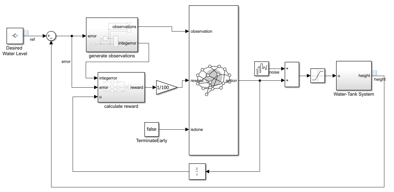
The Water-Tank System in rlWatertankPITuningUseCase1 is shown below:

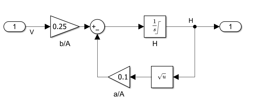
Here, $V$ is the voltage applied to the pump, and $H$ is the water level in the tank.

Define the observation specification obsInfo and the action specification actInfo.

obsInfo = rlNumericSpec([2 1]);
obsInfo.Name = 'observations';
obsInfo.Description = 'integrated error and error';

actInfo = rlNumericSpec([1 1]);
actInfo.Name = 'PID output';
actInfo.LowerLimit =  0;
actInfo.UpperLimit = 12;

Create an environment object from the modified water tank model, using rlSimulinkEnv.

mdl = 'rlWatertankPITuningUseCase1';
env = rlSimulinkEnv(mdl,[mdl '/RL Agent'],obsInfo,actInfo);

Set a custom reset function that randomizes the reference value and the initial water level for the model. To set the reset function, use the helper function localResetFcn, which is defined at the end of this example.

env.ResetFcn = @(in)localResetFcn(in,mdl);

From the observation and action specifications, extract the observation and action dimensions for this environment. Use prod(obsInfo.Dimension) and prod(actInfo.Dimension) to obtain the number of dimensions of the observation and action spaces, respectively, regardless of whether they are arranged as row vectors, column vectors, or matrices.

numObs = prod(obsInfo.Dimension);
numAct = prod(actInfo.Dimension);

Create RL Agent

To reproduce the results of this section, specify the seed and algorithm used for random number generation.

rng(0,"twister");

You can model a PI controller as linear policy. The policy uses both the error integral and the error as inputs, and outputs the control signal.

$$u=\left[\begin{array}{cc}\int e\text{dt}& e\end{array}\right]*{\left[\begin{array}{cc}{K}_i& K_p\end{array}\right]}^T$$

Here:

• u is the output of the policy.

• Ki and Kp (the integral and proportional gains of the PI controller) are the weights of the policy.

• The error signal is $e=\text{Href}-h\left(t\right)$, where $h\left(t\right)$ is the water level of the water in the tank, and $\text{Href}$ is the reference water level.

• During learning, the actor tunes the policy weights to minimize the cost.

To create the actor, use rlContinuousDeterministicActor with the basis function myBasisFcn, which is provided as a separate file in the example folder.

Display the file that implements the basis function.

type("myBasisFcn.m")

function feature = myBasisFcn(obs)
    % A basis function for Tune PI Controller Using Reinforcement Learning example
    
    % Copyright 2024 The MathWorks Inc.

    feature = obs;
end

Define the initial controller gains. Define Ki as 1e-3, and define Kp as 2.

initialGain = single([1e-3 2]);

Create the actor. For more information, see rlContinuousDeterministicActor.

actor = rlContinuousDeterministicActor( ...
    {@myBasisFcn,initialGain'},obsInfo,actInfo);

The agent in this example is a twin-delayed deep deterministic policy gradient (TD3) agent. TD3 agents rely on actor and critic approximator objects to learn the optimal policy. A TD3 agent approximates the long-term reward, given its observations and actions, by representing the value function (which approximates the cost function) with two-critics.

Create the critic networks using the function createCriticNet, which is defined in the following code section. Use the same network structure for both critics.

obsInputName = 'stateInLyr';
actInputName = 'actionInLyr';
criticNet1 = createCriticNet(numObs,numAct,obsInputName,actInputName);
criticNet2 = createCriticNet(numObs,numAct,obsInputName,actInputName);

function criticNet ...
        = createCriticNet(numObs,numAct,obsInputName,actInputName)
    statePath = [
        featureInputLayer(numObs,Name=obsInputName)
        fullyConnectedLayer(64,Name='fc1')
        ];

    actionPath = [
        featureInputLayer(numAct,Name=actInputName)
        fullyConnectedLayer(64,Name='fc2')
        ];

    commonPath = [
        concatenationLayer(1,2,Name='concat')
        reluLayer
        fullyConnectedLayer(64)
        reluLayer
        fullyConnectedLayer(1,Name='qvalOutLyr')
        ];

    criticNet = dlnetwork();
    criticNet = addLayers(criticNet,statePath);
    criticNet = addLayers(criticNet,actionPath);
    criticNet = addLayers(criticNet,commonPath);

    criticNet = connectLayers(criticNet,'fc1','concat/in1');
    criticNet = connectLayers(criticNet,'fc2','concat/in2');
end

Create the critic objects, using the specified neural network, the environment action and observation specifications, and the names of the network layers to be connected with the observation and action channels.

critic1 = rlQValueFunction(criticNet1, ...
    obsInfo,actInfo, ...
    ObservationInputNames=obsInputName, ...
    ActionInputNames=actInputName);

critic2 = rlQValueFunction(criticNet2, ...
    obsInfo,actInfo, ...
    ObservationInputNames=obsInputName,...
    ActionInputNames=actInputName);

Define a vector containing the critic objects.

critic = [critic1 critic2];

Specify the training options for the actor and critic. Set a relatively small learning rate to promote convergence, and set a gradient threshold to avoid drastic updates.

actorOpts = rlOptimizerOptions( ...
    LearnRate=5e-4, ...
    GradientThreshold=0.5);

criticOpts = rlOptimizerOptions( ...
    LearnRate=5e-4, ...
    GradientThreshold=0.5);

Specify the TD3 agent options using rlTD3AgentOptions.

• Set the agent to use the controller sample time Ts.

• Set the mini-batch size to 256 experience samples to reduce the variance when computing gradients.

• Set the experience buffer length to 1e6 to store a diverse set of experiences.

• Set the learning frequency to -1. This value means that the agent updates at the end of each episode.

• Set the max number of minibatches per epoch to 20 to reduce the number of gradient step updates for each learning iteration.

• Set the training options for the actor.

• Set the training options for the critic.

agentOpts = rlTD3AgentOptions( ...
    SampleTime=Ts, ...
    MiniBatchSize=256, ...
    DiscountFactor=0.99,...
    ExperienceBufferLength = 1e6, ...
    MaxMiniBatchPerEpoch = 20,...
    LearningFrequency = -1,...
    ActorOptimizerOptions=actorOpts, ...   
    CriticOptimizerOptions=criticOpts);

To modify the exploration model, use dot notation. Specifically, increase the standard deviation and its decay rate to promote exploration.

agentOpts.ExplorationModel.StandardDeviation = 0.5;
agentOpts.ExplorationModel.StandardDeviationDecayRate = 5e-5;

Set the standard deviation of the target policy smooth model to sqrt(0.1) to promote exploitation of actions with high Q-value estimates.

agentOpts.TargetPolicySmoothModel.StandardDeviation = sqrt(0.1);

Create the TD3 agent using the specified actor representation, critic representation, and agent options. For more information, see rlTD3Agent.

agent1 = rlTD3Agent(actor,critic,agentOpts);

Train RL Agent

Specify the random number stream for reproducibility.

rng(0,"twister");

Create an evaluator object to evaluate the performance of the agent over 10 simulations every 50 episodes. To apply different random initial conditions in each simulation, use the random seeds 1 through 10. The evaluation score is the average cumulative reward over the 10 evaluation episodes.

evaluatorObj = rlEvaluator("NumEpisodes",10,...
    "EvaluationFrequency",50,...
    "RandomSeeds",1:10);

To train the agent, first specify the following training options.

• Run each training for a maximum of 3000 episodes, with each episode lasting a maximum of 100 time steps.

• Display the training progress in the Reinforcement Learning Training Monitor (set the Plots option to "training-progress").

• Disable the command-line display (set the Verbose option as false).

• Stop the training when the evaluation score reaches -0.7. When the evaluation score reaches this level, the agent is capable of maintaining the water level at the reference value.

For more information on training options, see rlTrainingOptions.

maxepisodes = 3000;
maxsteps = ceil(Tf/Ts);
trainOpts = rlTrainingOptions( ...
    MaxEpisodes=maxepisodes, ...
    MaxStepsPerEpisode=maxsteps, ...
    ScoreAveragingWindowLength=100, ...
    Verbose=false, ...
    Plots="training-progress", ...
    StopTrainingCriteria="EvaluationStatistic", ...
    StopTrainingValue=-0.7);

Train the agent by using the train function. Training this agent is a computationally intensive process. To save time, load a pretrained agent by setting doTraining to false. To train the agent yourself, set doTraining to true.

doTraining = false;
if doTraining
    % Train the agent.
    trainingStats = train(agent1,env,trainOpts,Evaluator=evaluatorObj);
    save("WaterTankPITuningTD3AgentUseCase1.mat","agent1")
else
    % Load pretrained agent for the example.
    load("WaterTankPITuningTD3AgentUseCase1.mat","agent1")
end

Validate Trained Agent

To reproduce the results of this section, specify the seed and algorithm used for random number generation.

rng(0,"twister");

By default, the agent uses a greedy (hence deterministic) policy in simulation. If needed, you can use the exploratory policy instead, by setting the UseExplorationPolicy agent property to true.

To validate the trained agent, simulate it within the environment for a number of steps equal to maxsteps. For more information on agent simulation, see sim.

simOpts = rlSimulationOptions(MaxSteps=maxsteps);
experiences = sim(env,agent1,simOpts);

Show the cumulative reward obtained during the simulation episode.

sum(experiences.Reward.Data)

ans = 
-1.2940

The cumulative reward is close to the value obtained in the last training episodes, which suggests that the policy is able to stabilize the water level at the desired value.

Compare Performance of RL and Control System Tuner Gains

You can tune a controller in Simulink using Control System Tuner. To do so, you must specify the controller block as a tuned block, define the goals for the tuning process, and then on the Tuning tab, click Tune. For more information on using Control System Tuner, see Tune a Control System Using Control System Tuner (Simulink Control Design).

The values of the PI gains obtained using CST are as follows:

Kp_CST = 3.43726595858363;
Ki_CST = 0.0357784909005128;

The PI gains of the RL controller are the weights of the actor approximation model. To obtain the weights, first extract the learnable parameters from the actor.

actor = getActor(agent1);
parameters = getLearnableParameters(actor);

Obtain the controller gains.

Ki = parameters{1}(1)

Ki = single

0.1130

Kp = parameters{1}(2)

Kp = single

3.8090

Apply the gains obtained from the trained RL agent to the original PI controller block and run a step-response simulation.

First, open the unmodified water tank model.

open_system(WaterTankModel); 
set_param(WaterTankModel,"FastRestart","off")

Use the Simulink.SimulationInput (Simulink) object simIn to temporarily set the random seed for the noise, the reference water level and the initial water level, in the respective blocks.

refWaterLevel = 10;
initialWaterLevel = 1;
randomSeed = 1;
simIn = Simulink.SimulationInput(WaterTankModel);
noiseBlk = sprintf([WaterTankModel '/Band-Limited\nWhite Noise/']);
simIn = setBlockParameter(simIn,noiseBlk,'Seed',num2str(randomSeed));
refBlk = sprintf([WaterTankModel '/Desired \nWater Level']);
simIn = setBlockParameter(simIn,refBlk,'Value',num2str(refWaterLevel));
initBlk = [WaterTankModel '/Water-Tank System/H'];
simIn = setBlockParameter(simIn,initBlk,'InitialCondition',num2str(initialWaterLevel));

In the PID controller block, set the P and I parameter values to match the weights of the trained RL agent.

PIBlk = [WaterTankModel '/PID Controller'];
set_param([WaterTankModel '/PID Controller'],'P',num2str(Kp))
set_param([WaterTankModel '/PID Controller'],'I',num2str(Ki))

Use the Simulink sim function to simulate the water tank model with the applied temporary changes. The variable simResults that sim returns as output contains the fields simout and cost, which store the water level and cost recorded during the simulation. These fields are created by the two To Workspace blocks in the Simulink model.

simResults = sim(simIn);
rlStep1 = simResults.simout;
rlCost1 = simResults.cost;

Calculate the stability margin for the open-loop system by using the localStabilityAnalysis function, which is defined at the end of this example. The function returns a structure containing several stability margins, each one related to a snapshot of the system at a given time. Select a time of 50 seconds, which represents the midpoint of the 100-second simulation, when the system is expected to be near or at steady state.

blockIn  = [WaterTankModel '/Sum1'];
blockOut = [WaterTankModel '/Water-Tank System'];
stabilityAnalysisTime = 50;
rlStabilityMargin = localStabilityAnalysis(WaterTankModel,...
                                            blockIn,...
                                            blockOut,...
                                            stabilityAnalysisTime);

Apply the gains obtained using Control System Tuner to the original PI controller block and run a step-response simulation.

set_param([WaterTankModel '/PID Controller'],'P',num2str(Kp_CST))
set_param([WaterTankModel '/PID Controller'],'I',num2str(Ki_CST))

Use the Simulink sim function to simulate the water tank model with the PI gain values obtained from Control System Tuner. Collect the simulation results in simResult.

simResults = sim(simIn);
cstStep = simResults.simout;
cstCost = simResults.cost;

Calculate the stability margin for the open-loop system, using localStabilityAnalysis. Use the same stabilityAnalysisTime value of 50 seconds as for the RL controller.

cstStabilityMargin = localStabilityAnalysis(WaterTankModel,...
                                              blockIn,...
                                              blockOut,...
                                              stabilityAnalysisTime);

To analyze the step response for both simulations, use the stepinfo (Control System Toolbox) function.

rlStepInfo = stepinfo(rlStep1.Data,rlStep1.Time);
cstStepInfo = stepinfo(cstStep.Data,cstStep.Time);

Convert the structure returned from stepinfo (Control System Toolbox) into a table. Then remove unnecessary variables from the table, and add row names. For more information about table data type, see Tables.

stepInfoTable = struct2table([cstStepInfo rlStepInfo]);
stepInfoTable = removevars(stepInfoTable,{'SettlingMin', ...
    'TransientTime','SettlingMax','Undershoot','PeakTime'});
stepInfoTable.Properties.RowNames = {'CST','RL1'};

Display the step response table.

stepInfoTable

stepInfoTable = 2×4 table
           RiseTime    SettlingTime    Overshoot     Peak 
           ________    ____________    _________    ______

    CST     2.8482         3.896        0.75978     9.9904
    RL1     2.8737        12.582         2.7717     10.269

Convert the stability margin structures to tables.

stabilityMarginTable = struct2table( ...
    [cstStabilityMargin rlStabilityMargin]);

Remove unneeded variables, and add row names.

stabilityMarginTable = removevars(stabilityMarginTable,{...
    'GMFrequency','PMFrequency','DelayMargin','DMFrequency'});
stabilityMarginTable.Properties.RowNames = {'CST','RL1'};

Display the stability margin table.

stabilityMarginTable

stabilityMarginTable = 2×3 table
           GainMargin    PhaseMargin    Stable
           __________    ___________    ______

    CST      2.3401        67.134       true  
    RL1      2.1324        63.126       true  

Both controllers produce stable responses, with good (and comparable) gain and phase margins.

Compute the cumulative LQG costs for the two controllers.

rlCumulativeCost  = -sum(rlCost1.Data)

rlCumulativeCost = 
155.3710

cstCumulativeCost = -sum(cstCost.Data)

cstCumulativeCost = 
155.7214

The stability margin, and LQG cost results are comparable between the two tuning approaches. The step response rise times are also similar, while the CST gains provide much better overshoot and settling time.

Restore the random number stream using the information stored in previousRngState.

rng(previousRngState);

Local Functions

The localResetFcn function randomizes the reference signal and the initial water level.

function in = localResetFcn(in,mdl)
    % Randomize disturbance signal.
    randomSeed = randi(10000);
    noiseBlk = sprintf([mdl '/Band-Limited\nWhite Noise/']);
    in = setBlockParameter(in,noiseBlk,'Seed',num2str(randomSeed));

    % Randomize reference signal.
    hRef = 10 + 4*(rand-0.5);
    hRefBlk = sprintf([mdl '/Desired \nWater Level']);
    in = setBlockParameter(in,hRefBlk,'Value',num2str(hRef));

    % Randomize initial water level.
    hInit = 2*rand;
    hInitBlk = [mdl '/Water-Tank System/H'];
    in = setBlockParameter(in,hInitBlk,'InitialCondition',num2str(hInit));
end

The localStabilityAnalysis function computes stability margins by linearizing the closed-loop model at a specified time using loop-opening analysis points.

function margin = localStabilityAnalysis(mdl,blockIn,blockOut,time)
    set_param(mdl,"FastRestart","off")
    io(1) = linio(blockIn,1,'input');
    io(2) = linio(blockOut,1,'openoutput');
    op = operpoint(mdl);
    op.Time = time;
    linsys = linearize(mdl,io,op);
    margin =  allmargin(linsys);
end