tachorpm
Extract RPM signal from tachometer pulses
Description
[___] = tachorpm(
specifies options using name-value arguments and any of the previous
syntaxes.x,Fs,Name=Value)
tachorpm(___) with no output
arguments plots the generated RPM signal and the tachometer signal
with the detected pulses.
Examples
Load a simulated tachometer signal sampled at 300 Hz.
load tacho
Compute and visualize the RPM signal using tachorpm with the default values.
tachorpm(Yn,fs)

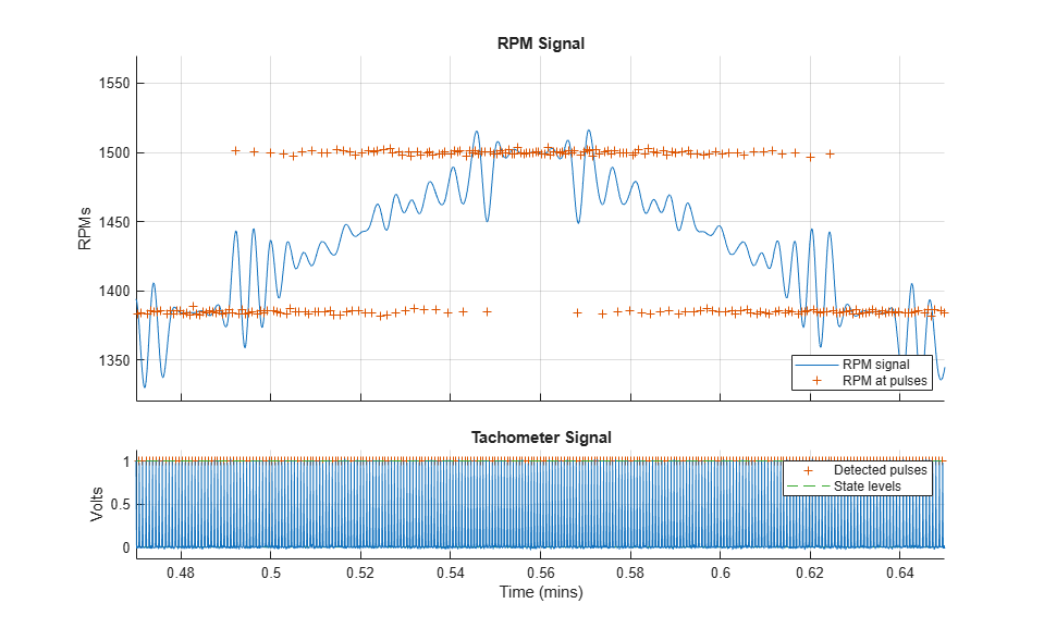
Increase the number of fit points to capture the RPM peak. Too many points result in overfitting. Verify this result by zooming in on the area around the peak.
tachorpm(Yn,fs,FitPoints=600)

axis([0.47 0.65 1320 1570])
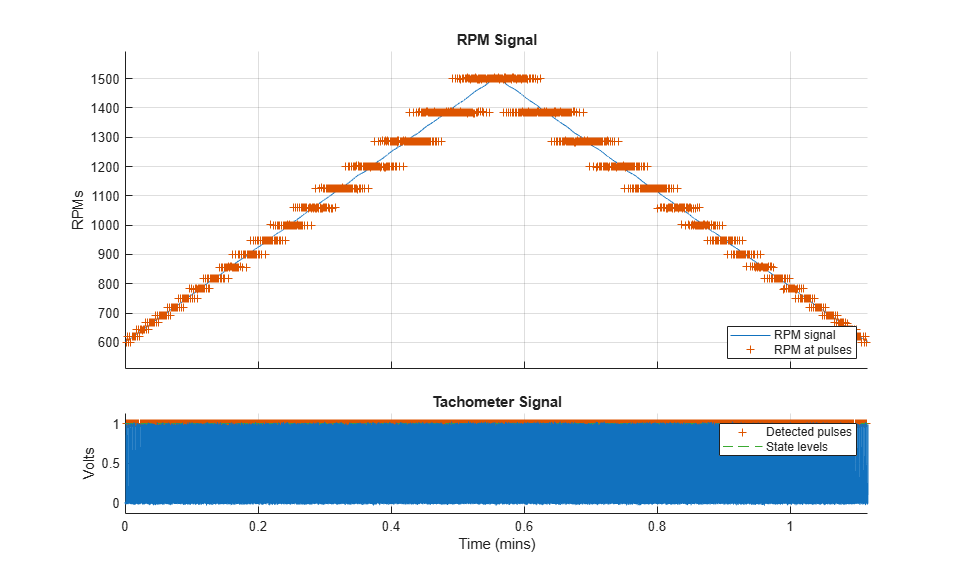
Choose a moderate number of points to obtain a better result.
tachorpm(Yn,fs,FitPoints=100)
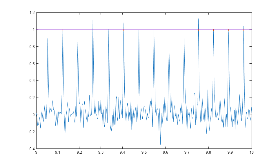
Add white Gaussian noise to the tachometer signal. The default pulse-finding mechanism misses pulses and returns a jagged signal profile. Verify this result by zooming in on a two-second time interval.
rng("default")
wgn = randn(size(Yn))/10;
Yn = Yn + wgn;

[rpm,t,tp] = tachorpm(Yn,fs,FitPoints=100);

figure
plot(t,Yn,tp,mean(interp1(t,Yn,tp))*ones(size(tp)),"+")
hold on
sl = statelevels(Yn);
plot(t,sl(1)*ones(size(t)),t,sl(2)*ones(size(t)))
hold off
xlim([9 10])
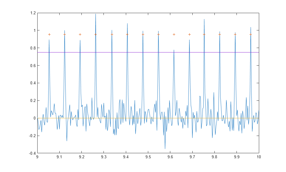
Adjust the state levels to improve the pulse finding.
sl = [0 0.75];

[rpm2,t,tp] = tachorpm(Yn,fs,FitPoints=100,StateLevels=sl);

plot(t,Yn,tp,mean(interp1(t,Yn,tp))*ones(size(tp)),"+")
hold on
plot(t,sl(1)*ones(size(t)),t,sl(2)*ones(size(t)))
hold off
xlim([9 10])
Input Arguments
Name-Value Arguments
Output Arguments
Algorithms
The tachorpm function performs these steps:
Uses
statelevelsto determine the low and high states of the tachometer signal.Uses
risetimeandfalltimeto find the times at which each pulse starts and ends. It then averages these readings to locate the time of each pulse.Note
The
tachorpmfunction detects rising and falling edges independently and in pairs, and without assuming whether a rising or falling edge occurs first along the tachometer signal. If a pulse starts mid-cycle –for example, when the high state follows a rising-falling-rising edge pattern but the signal begins with a falling edge– the function might pair the edges incorrectly. To make sure that the function calculates the RPM accurately in such cases, trim the tachometer signal so its first edge is a rising edge marking the start of a full pulse cycle.Uses
diffto determine the time intervals between pulse centers and computes the RPM values at the interval midpoints using RPM = 60 / Δt.If
FitTypeis specified as"smooth", then the function performs least-squares fitting usingspline. IfFitTypeis specified as"linear", then the function performs linear interpolation usinginterp1.
References
[1] Brandt, Anders. Noise and Vibration Analysis: Signal Analysis and Experimental Procedures. Chichester, UK: John Wiley & Sons, 2011.
[2] Vold, Håvard, and Jan Leuridan. “High Resolution Order Tracking at Extreme Slew Rates Using Kalman Tracking Filters.” Shock and Vibration. Vol. 2, 1995, pp. 507–515.
Extended Capabilities
Version History
Introduced in R2016b
See Also
orderspectrum | ordertrack | orderwaveform | rpmfreqmap | rpmordermap | rpmtrack | statelevels