glmval
Generalized linear model values
Syntax
Description
[
also computes 95% confidence bounds for the predicted values. ypred,yLo,yUp] = glmval(b,Xnew,Link,stats)stats is a
structure returned by the glmfit function. yLo and
yUp define a lower confidence bound of ypred-yLo,
and an upper confidence bound of ypred+yUp. Confidence bounds are
nonsimultaneous by default, and apply to the fitted curve, not to a new observation.
[___] = glmval(___,Name=Value) specifies
options using one or more name-value arguments in addition to any of the input argument
combinations in previous syntaxes. For example, you can specify the confidence level for the
confidence bounds.
Examples
Generate sample data using Poisson random numbers with two underlying predictors X(:,1) and X(:,2).
rng(0,"twister") % For reproducibility
rndvars = randn(100,2);
X = [2 + rndvars(:,1),rndvars(:,2)];
mu = exp(1 + X*[1;2]);
y = poissrnd(mu);
Fit a generalized linear regression model to the sample data.
b = glmfit(X,y,"poisson");b is a 3-by-1 vector of regression coefficients.
Create data points for prediction.
[Xtest1,Xtest2] = meshgrid(-1:.5:3,-2:.5:2);
Xnew = [Xtest1(:),Xtest2(:)];
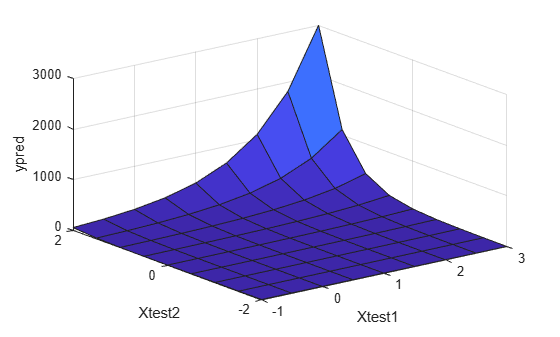
Predict the responses at the data points using the fitted model. Use the log link function, which is appropriate for a Poisson distribution.
ypred = glmval(b,Xnew,"log");Plot the predictions.
surf(Xtest1,Xtest2,reshape(ypred,9,9))
xlabel("Xtest1")
ylabel("Xtest2")
zlabel("ypred")
Fit a generalized linear regression model, and compute predicted (estimated) values for the predictor data using the fitted model.
Create a sample data set.
x = [2100 2300 2500 2700 2900 3100 ...
     3300 3500 3700 3900 4100 4300]';
n = [48 42 31 34 31 21 23 23 21 16 17 21]';
y = [1 2 0 3 8 8 14 17 19 15 17 21]';
x contains the predictor variable values. Each y value is the number of successes in the corresponding number of trials in n.
Fit a probit regression model for y on x using a binomial distribution for y.
b = glmfit(x,[y n],"binomial",Link="probit");
b is a 2-by-1 vector of regression coefficients.
Compute the estimated number of successes.
ypred = glmval(b,x,"probit",BinomialSize=n);Plot the observed and estimated percent success fractions versus the x values.
plot(x,y./n,"o",x,ypred./n,"-")
xlabel("x")
ylabel("Success Fraction")

Create a sample data set.
x = [2100 2300 2500 2700 2900 3100 ...
     3300 3500 3700 3900 4100 4300]';
n = [48 42 31 34 31 21 23 23 21 16 17 21]';
y = [1 2 0 3 8 8 14 17 19 15 17 21]';
x contains the predictor variable values. Each y value is the number of successes in the corresponding number of trials in n.
Define three function handles, created by using @, that define the link, the derivative of the link, and the inverse link for a probit link function. Store the function handles in a structure.
link = @(mu) norminv(mu);
derlink = @(mu) 1 ./ normpdf(norminv(mu));
invlink = @(resp) normcdf(resp);
F = struct(Link=link,Derivative=derlink,Inverse=invlink);
Fit a generalized linear model for y on x using a binomial distribution for y and the link function that you defined.
b = glmfit(x,[y n],"binomial",F);b is a 2-by-1 vector of regression coefficients.
Compute the estimated number of successes.
ypred = glmval(b,x,F,BinomialSize=n);
Plot the observed and estimated percent success fractions versus the x values.
plot(x, y./n,"o",x,ypred./n,"-")
xlabel("x")
ylabel("Success fraction")

Train a generalized linear model, and then generate code from a function that classifies new observations based on the model. This example is based on the Use Custom-Defined Link Function example.
Enter the sample data.
x = [2100 2300 2500 2700 2900 3100 ...
     3300 3500 3700 3900 4100 4300]';
n = [48 42 31 34 31 21 23 23 21 16 17 21]';
y = [1 2 0 3 8 8 14 17 19 15 17 21]';
Suppose that the inverse normal pdf is an appropriate link function for the problem.
Define a function named myInvNorm.m that accepts values of  and returns corresponding values of the inverse of the standard normal cdf.
function in = myInvNorm(mu) %#codegen
%myInvNorm Inverse of standard normal cdf for code generation
%   myInvNorm is a GLM link function that accepts a numeric vector mu, and
%   returns in, which is a numeric vector of corresponding values of the
%   inverse of the standard normal cdf.
%
in = norminv(mu);
end
Define another function named myDInvNorm.m that accepts values of and returns corresponding values of the derivative of the link function.
function din = myDInvNorm(mu) %#codegen
%myDInvNorm Derivative of inverse of standard normal cdf for code
%generation
%   myDInvNorm corresponds to the derivative of the GLM link function
%   myInvNorm. myDInvNorm accepts a numeric vector mu, and returns din,
%   which is a numeric vector of corresponding derivatives of the inverse
%   of the standard normal cdf.
%
din = 1./normpdf(norminv(mu));
end
Define another function named myInvInvNorm.m that accepts values of and returns corresponding values of the inverse of the link function.
function iin = myInvInvNorm(mu) %#codegen
%myInvInvNorm Standard normal cdf for code generation
%   myInvInvNorm is the inverse of the GLM link function myInvNorm.
%   myInvInvNorm accepts a numeric vector mu, and returns iin, which is a
%   numeric vector of corresponding values of the standard normal cdf.
%
iin = normcdf(mu);
end
Create a structure array that specifies each of the link functions. Specifically, the structure array contains fields named 'Link', 'Derivative', and 'Inverse'. The corresponding values are the names of the functions.
link = struct('Link','myInvNorm','Derivative','myDInvNorm',...
    'Inverse','myInvInvNorm')
link =

  struct with fields:

          Link: 'myInvNorm'
    Derivative: 'myDInvNorm'
       Inverse: 'myInvInvNorm'
Fit a GLM for y on x using the link function link. Return the structure array of statistics.
[b,~,stats] = glmfit(x,[y n],'binomial','link',link);
b is a 2-by-1 vector of regression coefficients.
In your current working folder, define a function called classifyGLM.m that:
Accepts measurements with columns corresponding to those in
x, regression coefficients whose dimensions correspond tob, a link function, the structure of GLM statistics, and any validglmvalname-value pair argumentReturns predictions and confidence interval margins of error
function [yhat,lo,hi] = classifyGLM(b,x,link,varargin) %#codegen
%CLASSIFYGLM Classify measurements using GLM model
%   CLASSIFYGLM classifies the n observations in the n-by-1 vector x using
%   the GLM model with regression coefficients b and link function link,
%   and then returns the n-by-1 vector of predicted values in yhat.
%   CLASSIFYGLM also returns margins of error for the predictions using
%   additional information in the GLM statistics structure stats.
narginchk(3,Inf);
if(isstruct(varargin{1}))
    stats = varargin{1};
    [yhat,lo,hi] = glmval(b,x,link,stats,varargin{2:end});
else
    yhat = glmval(b,x,link,varargin{:});
end
end
Generate a MEX function from classifyGLM.m. Because C uses static typing, codegen must determine the properties of all variables in MATLAB® files at compile time. To ensure that the MEX function can use the same inputs, use the -args argument to specify the following in the order given:
Regression coefficients
bas a compile-time constantIn-sample observations
xLink function as a compile-time constant
Resulting GLM statistics as a compile-time constant
Name
'Confidence'as a compile-time constantConfidence level 0.9
To designate arguments as compile-time constants, use coder.Constant.
codegen -config:mex classifyGLM -args {coder.Constant(b),x,coder.Constant(link),coder.Constant(stats),coder.Constant('Confidence'),0.9}
Code generation successful.
codegen generates the MEX file classifyGLM_mex.mexw64 in your current folder. The file extension depends on your system platform.
Compare predictions by using glmval and classifyGLM_mex. Specify name-value pair arguments in the same order as in the -args argument in the call to codegen.
[yhat1,melo1,mehi1] = glmval(b,x,link,stats,'Confidence',0.9);
[yhat2,melo2,mehi2] = classifyGLM_mex(b,x,link,stats,'Confidence',0.9);

comp1 = (yhat1 - yhat2)'*(yhat1 - yhat2);
agree1 = comp1 < eps
comp2 = (melo1 - melo2)'*(melo1 - melo2);
agree2 = comp2 < eps
comp3 = (mehi1 - mehi2)'*(mehi1 - mehi2);
agree3 = comp3 < eps
agree1 =

  logical

   1


agree2 =

  logical

   1


agree3 =

  logical

   1
The generated MEX function produces the same predictions as predict.
Input Arguments
Name-Value Arguments
Output Arguments
References
[1] Dobson, A. J. An Introduction to Generalized Linear Models. New York: Chapman & Hall, 1990.
[2] McCullagh, P., and J. A. Nelder. Generalized Linear Models. New York: Chapman & Hall, 1990.
[3] Collett, D. Modeling Binary Data. New York: Chapman & Hall, 2002.
Extended Capabilities
Version History
Introduced before R2006a