rectangularPulse
Rectangular pulse function
Description
Examples
Compute the rectangular pulse function at coordinates –2, –1, 0, 1, and 2 with specified rising and falling edge at –1 and 1. Because these inputs are not symbolic objects, you get floating-point results.
r = rectangularPulse(-1,1,-2:2)
r = 1×5

         0    0.5000    1.0000    0.5000         0
Compute the rectangular pulse function for the same inputs in symbolic form.
r = rectangularPulse(sym(-1),1,-2:2)
r =
Plot the rectangular pulse function using fplot.
syms x
fplot(rectangularPulse(x), [-1 1])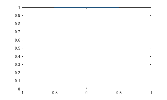
Show that if a < b, the rectangular pulse function for x = a and x = b equals 1/2.
syms a b x
assume(a < b)
r = rectangularPulse(a,b,a)
r =
r = rectangularPulse(a,b,b)
r =
For further computations, remove the assumptions on the variables a and b by recreating them using syms.
syms a b
For a = b, the rectangular pulse function returns 0.
r = rectangularPulse(a,a,x)
r =
The default value of the rectangularPulse function at the rising and falling edges is 1/2.
syms a b
assume(a < b)
r = rectangularPulse(a,b,a)
r =
r = rectangularPulse(a,b,b)
r =
Another common value at these edges is 1. To change the value of rectangularPulse at the edges, use sympref to set the value of the 'HeavisideAtOrigin' setting. Store the previous parameter value returned by sympref, so that you can restore it later.
oldparam = sympref('HeavisideAtOrigin',1);Check the new value of rectangularPulse at the rising and falling edges.
r = rectangularPulse(a,b,a)
r =
r = rectangularPulse(a,b,b)
r =
The settings you set using sympref persist throughout your current and future MATLAB® sessions. To restore the previous value of rectangularPulse at the edges, use the value stored in oldparam.
sympref('HeavisideAtOrigin',oldparam);Alternatively, you can restore the default value of 'HeavisideAtOrigin' by using the 'default' setting.
sympref('HeavisideAtOrigin','default');
When the rising or falling edge of rectangularPulse is at the infinity, then this function is the same as the Heaviside step function (the unit step function).
syms x
r = rectangularPulse(-Inf,0,x)
r =
r = rectangularPulse(0,Inf,x)
r =
Input Arguments
More About
Tips
Version History
Introduced in R2012b
See Also
dirac | heaviside | triangularPulse | sympref