HDL Implementation of Fading Channel
This example shows the implementation of a fading channel that is optimized for HDL code generation and hardware implementation [ 1 ]. This hardware implementation of fading channel can be used in the performance evaluation of wireless communication systems that undergoes Rayleigh and Rician fading channel environment. In this example, the Simulink® model accepts a Discrete path delays, Average power gains, Normalize average path gain and Fading distribution as property parameter in the mask along with the input modulated symbols and input valid through input port and gives out faded channel outputs along with valid signal.
Modern wireless communication systems include many different types of channel models such as pedestrian-A, pedestrian-B, vehicular, and ETU. The performance evaluation of these systems with these channel models is a bottleneck. Hardware capabilities of FPGAs can speed up simulations.
Model Architecture
% Run this command to open the HDLFadingChannel model.
modelname = 'HDLFadingChannel';
open_system(modelname);

The top-level structure of the model includes these two subsystems.
Generate complex channel coefficients
Perform FIR filtering
% Run this command to open the subsystems inside SISO Fading Channel model.
open_system([modelname '/SISO Fading Channel'],'force');

Generate complex channel coefficients
The Generate complex channel coefficients subsystem generates the complex channel coefficients which is used in the discrete FIR filter. This subsystem internally has three subsystems shown below
open_system([modelname '/SISO Fading Channel/Generate complex channel coefficients']);

*Generate multiplication and addition factor – this subsystem, calculates the multiplication factor and addition factor. This subsystem has two sections namely
The Calculate multiplication and addition factor section accepts the Discrete path delay, Average path gains, Normalization check box, Fading distribution, Kfactor from the mask parameter and validIn through input port. This section calculates and gives out the mulFacVector and addFacVector factor vector corresponding to the discrete path delays vector.
The Select multiplication and addition factor section selects mulFacScalar and addFacScalar from the mulFacVector and addFacVector respectively based on the countPathDelays.
open_system([modelname '/SISO Fading Channel/Generate complex channel coefficients/Generate multiplication and addition factor']);

*Generate gaussian random variables – this subsystem, generates two Gaussian random variates one for real part another for imaginary part using Box-Muller approach.
*Form the complex channel – this subsystem consists of three sections shown below
The DTC as input section converts the data type of dataInGaussRe and dataInGaussRe signal into the input data type.
The Multiplying with multiplication factor section multiplies the dataGaussRe and dataGaussIm signal with MF (multiplication factor) signal and outputs the complex coefficients.
The Adding the addition factor section adds the AF (addition factor) signal to the complex coefficients from the previous section and output the complxChanCoeff signal.
open_system([modelname '/SISO Fading Channel/Generate complex channel coefficients/Form the complex channel']);

Perform FIR filtering
The Perform FIR filtering subsystem filters the input data with the generated complex channel coefficients and gives out the faded symbols. This subsystem consists of these sections:
The Convert scalar channel to vector section converts the scalar channel coefficients chanScalIn to vector channel coefficients chanVecOut.
The Filter input data with channel coefficients section filters the input data with the vector complex channel coefficients using Discrete FIR filter block to give the faded output symbols.
open_system([modelname '/SISO Fading Channel/Perform FIR filtering']);

Set Up Mask Variables
For Discrete path delays (samples), user can give non-negative integers in the ascending order. Each value indicates the relative delay of samples from the first path. Discrete path delays in samples can be calculated by multiplying path delay in seconds by sampling rate.
For _Average path gains (in dB), user can give real numbers.
If user requires to normalize the gain, Normalize average path gains to 0 dB check box can be checked otherwise it can be unchecked.
User can select the Fading distribution drop down either to 'Rayleigh' or 'Rician'
k-factor edit box appears only when user selects the Fading distribution to 'Rician'. When user sets k-factor to a scalar, the first discrete path is a Rician fading process with that k-factor value. Any remaining discrete paths are independent Rayleigh fading processes. When user sets k-factor to a vector, the discrete path corresponding to a positive element of the k-factor vector is a Rician fading process with k-factor specified by that element. The discrete path corresponding to any zero-valued elements of the k-factor vector are Rayleigh fading processes.
discretePathDelays =  [0     2     4      8]; % Discrete path delays (samples)
avgPathGainsdB     =  [0    -3    -6    -12]; % Average path gains (in dB)
normAvgPowTo0dB    =  true;                   % Normalize average path gains to 0 dB
fadingDistri = 'Rician';                      % Fading distribution: 'Rayleigh' or 'Rician'
if strcmp(fadingDistri,'Rician')
    KFactor = [ 3 0 0 2.5];                   % k-factor with value 0 will be Rayleigh distributed
else
    KFactor = 0;                              % k-factor
end
if normAvgPowTo0dB
    set_param('HDLFadingChannel/SISO Fading Channel','normPathGain','on')
else
    set_param('HDLFadingChannel/SISO Fading Channel','normPathGain','off') %#ok<UNRCH>
end
set_param('HDLFadingChannel/SISO Fading Channel','fadingDistri',fadingDistri)
Generate Input Data and Run Simulink Model
numSymbols = 10^(6);% number of modulated input symbols
modOrder = 4; % order of modulation
symMap = [0 2 3 1]; % symbol mapping
phaseOffset = pi/4; % phase offset
nBitsPerSym = log2(modOrder); % number of bits per symbol
numBits = numSymbols*nBitsPerSym; % total number of input bits used
inpBits = randi([0 1],numBits,1); % input bit generation.
dataInSym = pskmod(inpBits, modOrder, phaseOffset, symMap, 'InputType', 'bit'); % input symbols to the example
validInSym = boolean([ones(1,numSymbols)]); % input valid to the example
simTime = numSymbols+1000;

% Simulate the model
out = sim('HDLFadingChannel');

% Collect the faded output symbols
fadedComplxSym = out.fadedChanDataOut(out.fadedChanValidOut);
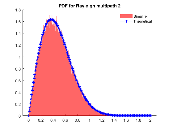
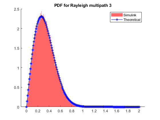
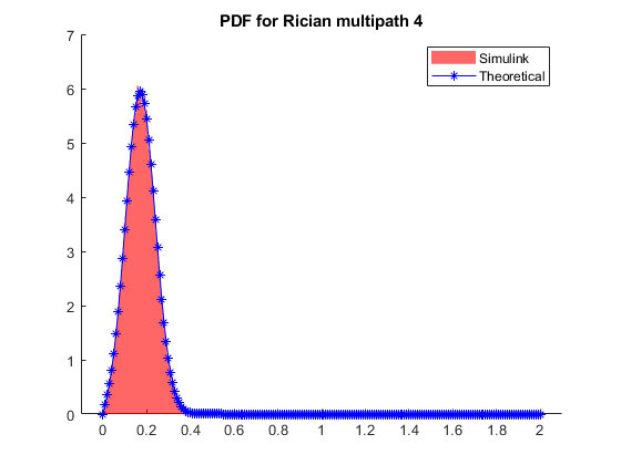
Verify Channel Fading Distribution
squeezeChOut = squeeze(out.chScalar);
repmatChValid = squeeze(out.chScalarValid);
reqdChValid = repmatChValid.';
chCoeff = squeezeChOut(boolean(reqdChValid));
[chCoeffRows, ~ ] = size(chCoeff);
chanMatRowSize = floor(chCoeffRows/(discretePathDelays(end)+1));
chanSize = chanMatRowSize * (discretePathDelays(end)+1);
chanCoeffOut = reshape(chCoeff(1:chanSize),(discretePathDelays(end)+1),chanMatRowSize).';

pathGainlin=10.^(avgPathGainsdB/10);
if normAvgPowTo0dB
    avgPowLin=pathGainlin/sum(pathGainlin);
else
    avgPowLin=pathGainlin; %#ok<UNRCH>
end

% Plot PDF
fadProbDist = get_param('HDLFadingChannel/SISO Fading Channel','fadingDistri');
if strcmp(fadProbDist,'Rician')
    if length(KFactor) < length(discretePathDelays)
        KFactor = [KFactor zeros(1,length(discretePathDelays)-length(KFactor))];
    end
    for pathNum = 1:length(discretePathDelays)
        if KFactor(pathNum)
            fadStr = 'Rician';
        else
            fadStr = 'Rayleigh';
        end
        figure (pathNum)
        str = sprintf('PDF for %s multipath %d',fadStr,pathNum);
        title(str)
        hold on
        histogram(abs(chanCoeffOut(:,discretePathDelays(pathNum)+1)),500,...
            'Normalization','pdf','BinLimits',[0 2],'FaceColor','red', ...
            'EdgeColor','none');
        x = (0:0.01:2);
        p = pdf('Rician',x,sqrt(avgPowLin(pathNum)*KFactor(pathNum)/(KFactor(pathNum)+1)),sqrt(avgPowLin(pathNum)/(2*(KFactor(pathNum)+1))));
        plot(x,p,'-b*')
        str1 = sprintf('Simulink');
        str2 = sprintf('Theoretical');
        legend(str1,str2)
    end
else
    for pathNum = 1:length(discretePathDelays)
        figure (pathNum)
        str = sprintf('PDF for Rayleigh multipath %d',pathNum);
        title(str)
        hold on
        histogram(abs(chanCoeffOut(:,discretePathDelays(pathNum)+1)),500,...
            'Normalization','pdf','BinLimits',[0 2],'FaceColor','blue', ...
            'EdgeColor','none');
        x = (0:0.01:2);
        p = raylpdf(x,sqrt(avgPowLin(pathNum)/2));
        plot(x,p,'-r*')
        str1 = sprintf('Simulink');
        str2 = sprintf('Theoretical');
        legend(str1,str2)
    end
end

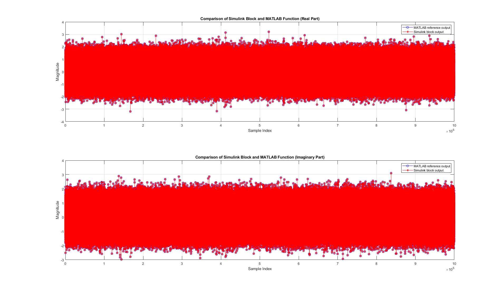
Verify Channel Output
Compare the output of the Fading Simulink model with the output of the HDL equivalent fading channel MATLAB function.
% MATLAB output
fprintf('\n Simulating MATLAB HDL Fading for comparison...\n');
fadedComplxSymMatlab = hdlFadingChan(dataInSym,discretePathDelays,avgPathGainsdB,normAvgPowTo0dB,fadingDistri,KFactor);
fprintf('\n Simulation complete. \n')

% Compare MATLAB and Simulink outputs
figure('units','normalized','outerposition',[0 0 1 1])
subplot(2,1,1)
plot(real(fadedComplxSymMatlab(:)),'-bo');
hold on;
plot(real(fadedComplxSym(:)),'-r*');
grid on
legend('MATLAB reference output','Simulink block output')
xlabel('Sample Index')
ylabel('Magnitude')
title('Comparison of Simulink Block and MATLAB Function (Real Part)')

subplot(2,1,2)
plot(imag(fadedComplxSymMatlab(:)),'-bo');
hold on;
plot(imag(fadedComplxSym(:)),'-r*');
grid on
legend('MATLAB reference output','Simulink block output')
xlabel('Sample Index')
ylabel('Magnitude')
title('Comparison of Simulink Block and MATLAB Function (Imaginary Part)')

sqnrRealdB = 10*log10(double(var(real(fadedComplxSym(:)))/abs(var(real(fadedComplxSym(:)))-var(real(fadedComplxSymMatlab(:))))));
sqnrImagdB = 10*log10(double(var(imag(fadedComplxSym(:)))/abs(var(imag(fadedComplxSym(:)))-var(imag(fadedComplxSymMatlab(:))))));

fprintf('\n HDL Fading Channel output \n SQNR of real part: %.2f dB',sqnrRealdB);
fprintf('\n SQNR of imaginary part: %.2f dB\n',sqnrImagdB);
 Simulating MATLAB HDL Fading for comparison...

 Simulation complete.

 HDL Fading Channel output
 SQNR of real part: 38.74 dB
 SQNR of imaginary part: 38.69 dB
HDL Code Generation
To check and generate the HDL code referenced in this example, you must have an HDL Coder (TM) license.
To generate the HDL code, enter this command at the MATLAB command prompt.
makehdl('HDLFadingChannel/SISO Fading Channel')
To generate a test bench, enter this command at the MATLAB command prompt.
makehdltb('HDLFadingChannel/SISO Fading Channel')
Synthesize the HDLFadingChannel subsystem on a Xilinx Zynq® UltraScale+ RFSoC xczu29dr-ffvf1760-2-e. This table shows the resource utilization results.
F = table(...
    categorical({'Slice LUT';'Slice Registers';'RAMB36';'DSP'; ...
    'Max. Frequency (MHz)'}) ,...
    categorical({'9269';'8279';'4';'56';'322.55'}), ...
    'VariableNames',{'Resources','Values'});

disp(F);
         Resources          Values
    ____________________    ______

    Slice LUT               9269
    Slice Registers         8279
    RAMB36                  4
    DSP                     56
    Max. Frequency (MHz)    322.55
References
A. Alimohammad, S. F. Fard and B. F. Cockburn, "Hardware Implementation of Rayleigh and Ricean Variate Generators," in IEEE Transactions on Very Large Scale Integration (VLSI) Systems, vol. 19, no. 8, pp. 1495-1499, Aug. 2011, doi: 10.1109/TVLSI.2010.2051465.