Radar Target Emulation on NI USRP Radio

Since R2025a

This example shows how to deploy a radar target emulation algorithm on the FPGA of an NI™ USRP™ radio.

Workflow

In this example, you follow a step-by-step guide to generate a custom FPGA image from a Simulink^® model and deploy it on an NI USRP radio.

You can use the deployed target emulation design to test various radar scenarios using real world signals. These examples provide host interface scripts that enable you to exercise and verify the deployed design in different deployment scenarios. The table gives an overview. For more information, see Radar Target Emulation Applications Overview.

Example	Deployment Test Scenario
Pulse Radar Scenario Using Target Emulator on NI USRP Radio	Run a pulse radar scenario on an NI USRP radio with the target emulation algorithm deployed on the FPGA. Use the same radio to transmit a linear FM radar pulse train, then capture and plot the emulated target range-Doppler response in MATLAB.
Real Time Target Emulation on NI USRP Radio	Run a pulse radar scenario on an NI USRP radio with the target emulation algorithm deployed on the FPGA, running continuously. Use a second NI USRP radio to transmit a linear FM radar pulse train, then capture and plot the emulated target range-Doppler response in MATLAB.
Integrated Sensing and Communication Using 6G Waveform on NI USRP Radio	Generate a 6G waveform to track a moving object in an integrated sensing and communications (ISAC) scenario. Use the same radio to transmit the generated waveform, then capture and plot the emulated target range-Doppler response in MATLAB.

For more information about how to prototype and deploy software-defined radio (SDR) algorithms on the FPGA of an NI USRP radio, see Target NI USRP Radios Workflow.

Design Overview

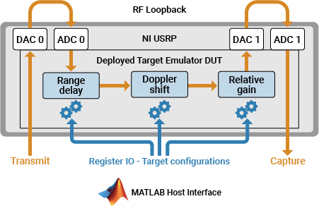
The example uses the algorithm from the Radar Target Emulator with HDL Coder (Radar Toolbox) example. The algorithm receives a linear FM pulse train and emulates up to eight targets by applying variable range delays, Doppler shifts, and gains to the received waveform. Then, the algorithm retransmits the modified waveform at a known time offset. This design modifies the interfaces that enable you to deploy the generated bitstream on the FPGA of an NI USRP radio.

Requirements

To target NI USRP radio devices with Wireless Testbench™, you must install and configure third-party tools and additional support packages.

For details about which NI USRP radios you can target, see Supported Radio Devices.

Note

Generating a bitstream with this workflow is supported only on a Linux^® operating system (OS). For details about host system requirements, see System Requirements.

For details about how to install and configure additional support packages and third-party tools, see Installation for Targeting NI USRP Radios.

Note

You cannot use this example with a USRP X310 radio with TwinRX daughterboards because it requires a transmit path.

Set Up Environment and Radio

Set up a working directory for running the example by using the openExample function in MATLAB^®. This function downloads the example files into a subfolder of the Examples folder in the currently running release and then opens the example. If a copy of the example exists, openExample opens the existing version of the example.

openExample('wt/USRPRADARTargetEmulatorExample')

The working directory contains all the files you need to use this example, including helper functions and files. The files you interact with are:

• wtRADARTargetEmulatorSL.slx — The Simulink hardware generation model. This model includes the DUT subsystem, which implements a radar target emulation algorithm, and additional subsystems than enable you to simulate the DUT behavior.

• RadarTargetEmulationOnNISRPRadioExample.m — The MATLAB script that you can use to simulate the behavior of the Simulink model before you generate HDL code.

• VerifyRadarTargetEmulatorAlgorithmUsingMATLABExample.m — A live script that you can use in MATLAB to verify the algorithm running your radio.

To program the FPGA on your radio with the bitstream that you generate in this example, and to verify the algorithm running on your radio, use the Radio Setup wizard to connect and set up your radio.

Simulink Hardware Generation Model

The Simulink model in this example implements the target emulation algorithm using a hardware modeling style and uses blocks that support HDL code generation. The model uses fixed-point arithmetic and includes control signals that control the flow of data through the model.

Open Model

Open the Simulink model.

open_system('wtRADARTargetEmulatorSL');

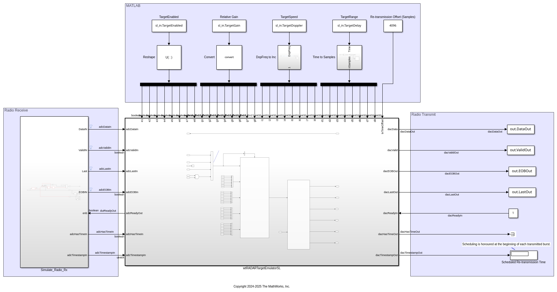
The top-level structure of the model includes the wtRADARTargetEmulatorSL subsystem, which is the DUT. In addition, it contains subsystems and blocks that generate input data and save output data for simulating the behavior of the DUT model.

Open the wtRADARTargetEmulatorSL subsystem.

open_system('wtRADARTargetEmulatorSL/wtRADARTargetEmulatorSL');

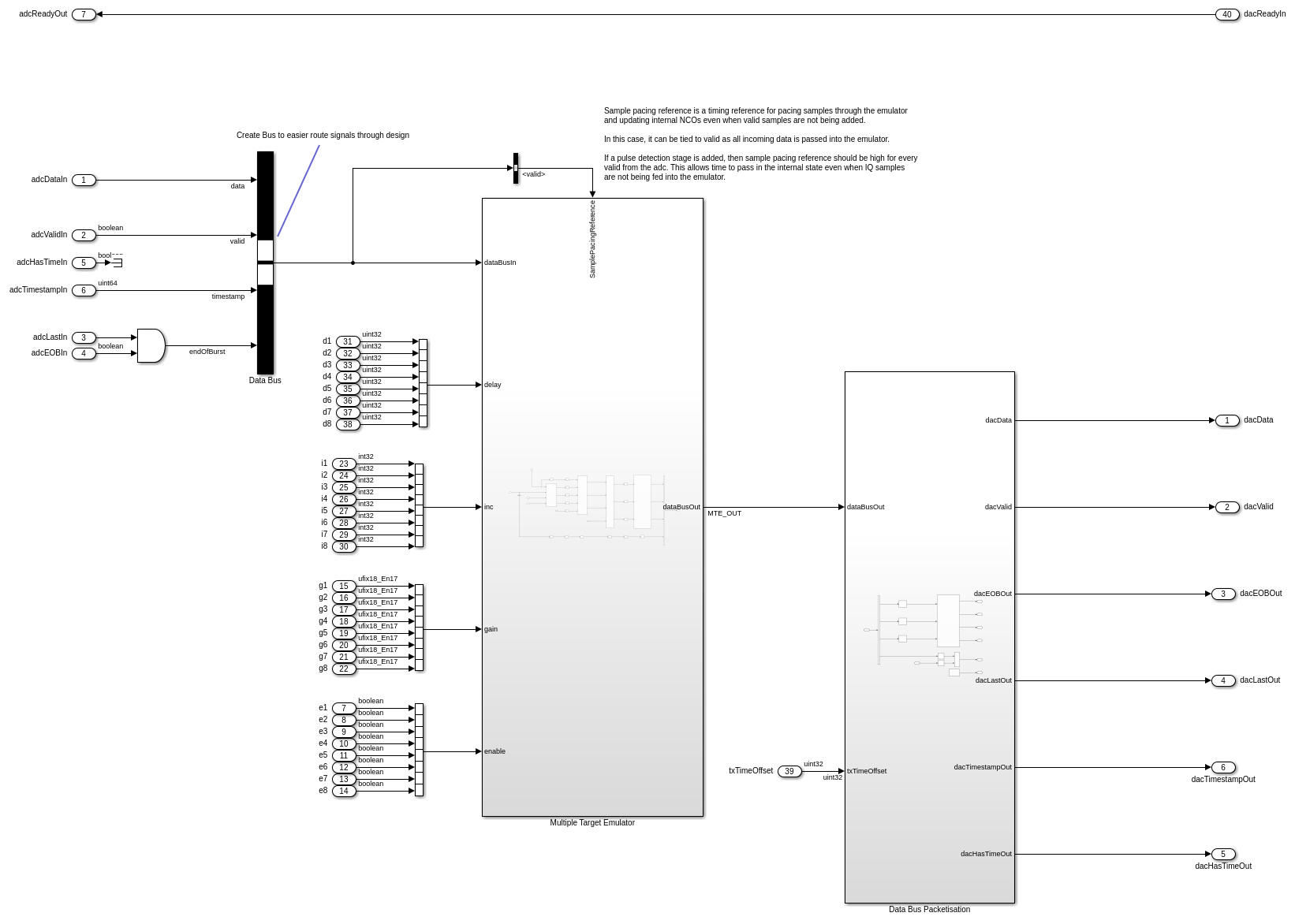
Data flows through these blocks and subsystems:

• The AND block asserts the end of burst (EOB) signal on the last sample of the last packet of each burst.

• The Multiple Target Emulator subsystem emulates the response of up to eight different targets.

• The Data Bus Packetisation subsystem implements the signaling for the streaming interface output.

Open the Multiple Target Emulator subsystem.

open_system('wtRADARTargetEmulatorSL/wtRADARTargetEmulatorSL/Multiple Target Emulator');

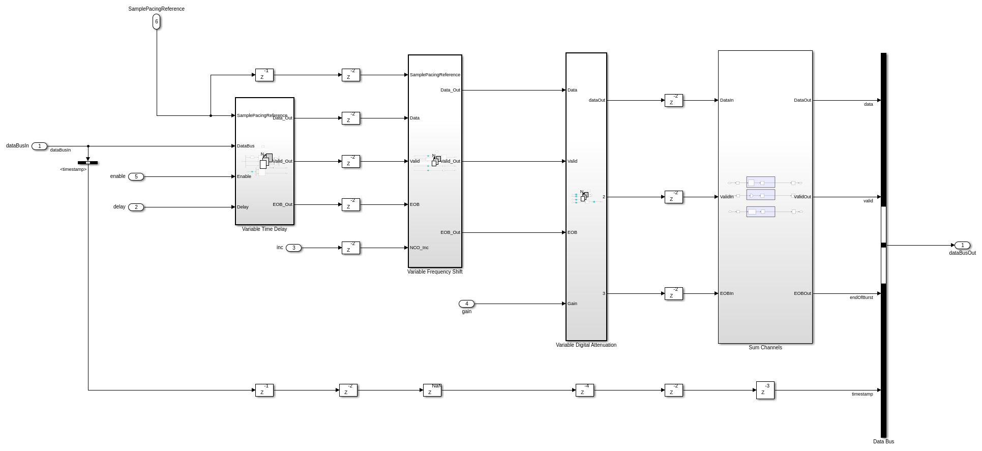
This subsystem emulates the response for eight different targets by applying a variable time delay, variable frequency shift, and variable attenuation according to the enable, delay, inc, and gain input ports. The operation is as follows:

1. When enable is true, the input data is provided to the variable time delay.

2. The variable time delay buffers the input samples in memory for the number of samples specified by the delay port.

3. The delayed data is multiplied by the output of an numerically controlled oscillator (NCO) to achieve a variable frequency shift. The NCO is controlled by the inc port value.

4. The delayed and shifted data is multiplied by the gain port value to achieve a variable attenuation.

5. The Sum Channels subsystem combines the responses from the eight targets into a single data stream.

6. The timestamp of the sample is delay balanced with the data path.

In the top-level subsystem, the inputs for each target are specified as input register ports on the wtRADARTargetEmulatorSL subsystem: e1 to e8 correspond to the enable input ports; d1 to d8 to the delay input ports; i1 to i8 to the inc input ports; and g1 to g8 to the gain input ports for each of the eight targets respectively.

Open the Data Bus Packetisation subsystem.

open_system('wtRADARTargetEmulatorSL/wtRADARTargetEmulatorSL/Data Bus Packetisation');

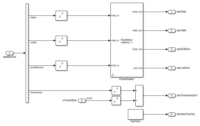
This subsystem implements the last, end of burst (EoB), has time, and timestamp signals for the data streaming output in.

The SPP input port defines the samples per packet, which is the number of valid samples between assertions of the last signal. If the SPP input value is zero, which is the default value of the register on the hardware, the SPP value defaults to 256. You can reduce round-trip latency of the target emulator by specifying a smaller value for the SPP input port from MATLAB. The optimal value depends on the specific hardware setup.

The txTimeOffset input sets the scheduled re-transmission time as an offset from the received timestamp. If the txTimeOffset input value is set to zero, the has time signal, dacHasTimeOut, is set low. This specifies that the transmission should be scheduled as soon as possible. Specifying a non-zero value for txTimeOffset input from MATLAB allows for precise sample-level control of the round-trip latency inside the FPGA. If the txTimeOffset value is too short, the burst may arrive late at the radio front end. If the txTimeOffset is longer than the available buffers allow, then overflows will occur due to backpressure. The optimal value varies depending on the specific hardware setup and value of the SPP input port.

Simulate Design

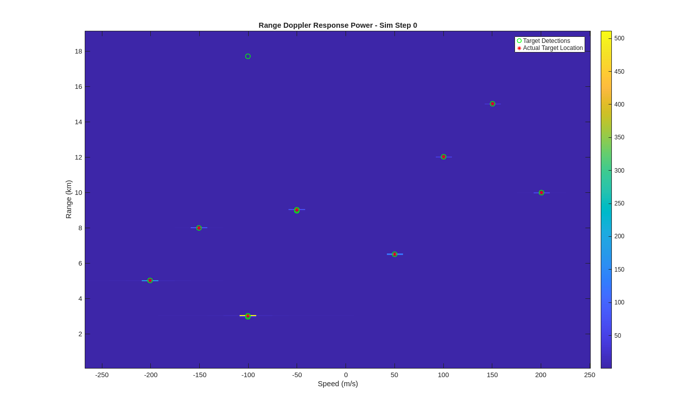
Verify the design by simulating the model. Enable the eight targets and specify the initial radar cross section (RCS), range, and speed.

targetEnabled = [true true true true true true true true]; % Set true to sim target
targetRCS = [1 4 1 2 3 2 4 3]; % dBsm
targetRange = [5e3 15e3 3e3 6.5e3 10e3 8e3 12e3 9e3]; % m
targetSpeed = [-200 150 -100 50 200 -150 100 -50]; % m/s

Set the maximum gain from which the relative gains applied by the model are calculated. This prevents unnecessary signal loss due to the fixed point data type and can be accounted for using the radio gain at the radio front end. Specify maxGain as empty to use the highest calculated real world gain in the helperRadarTargetSimulationSetup function.

maxGain = [];

Set the target emulation parameters used by the model in MATLAB by using the helperRadarTargetSimulationSetup function.

sl_in = helperRadarTargetSimulationSetup( ...
    targetEnabled,targetRCS,targetRange,targetSpeed,maxGain);

Simulate the model.

sl_out = sim("wtRADARTargetEmulatorSL.slx");

### Searching for referenced models in model 'wtRADARTargetEmulatorSL'.
### Total of 1 models to build.

Create a range-Doppler response object for processing data.

rdResponse = phased.RangeDopplerResponse(...
    'DopplerFFTLengthSource','Property', ...
    'DopplerFFTLength',sl_in.VelDimLen, ...
    'PRFSource','Property', 'PRF',sl_in.PRF,...
    'SampleRate',sl_in.Fs,'DopplerOutput','Speed', ...
    'OperatingFrequency',sl_in.Fc);

Create a two-dimensional CFAR detector object for detection generation.

cfar = phased.CFARDetector2D(GuardBandSize=[25 1],...
    TrainingBandSize=[10 1],...
    ProbabilityFalseAlarm=1e-4);

Process the simulation output data and plot the range-Doppler response using the helperVisualizeRadarTargetSimulation function.

fig = figure;
ax = axes(fig);
helperVisualizeRadarTargetSimulation(sl_out,sl_in,rdResponse,cfar,0,ax);

Configure IP Core

When you are satisfied with the simulated behavior of the model, you can proceed to integrate your design into a custom IP core by generating HDL code and mapping the model inputs and outputs to the hardware interfaces.

First, use the hdlsetuptoolpath (HDL Coder) function to set up the tool chain. Specify the path to your Vivado^® bin directory. For more information, see Set Up Third-Party Tools.

hdlsetuptoolpath('ToolName','Xilinx Vivado', ...
    'ToolPath','/opt/Xilinx/Vivado/2021.1/bin');

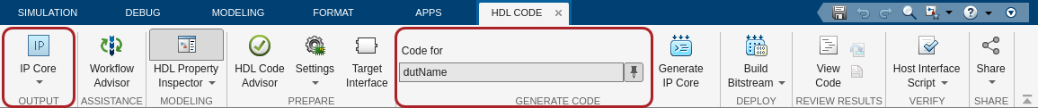
From the Apps tab in the Simulink Toolstrip, select HDL Coder. Then open the HDL Code tab.

Configure Output Options

In the HDL Code tab, configure the output options:

• Ensure the wtRADARTargetEmulatorSL subsystem is pinned in the Code for option. To pin this selection, select the wtRADARTargetEmulatorSL subsystem in the Simulink model and click the pin icon.

• Select IP Core as the Output > IP Core option.

Configure HDL Code Generation Settings

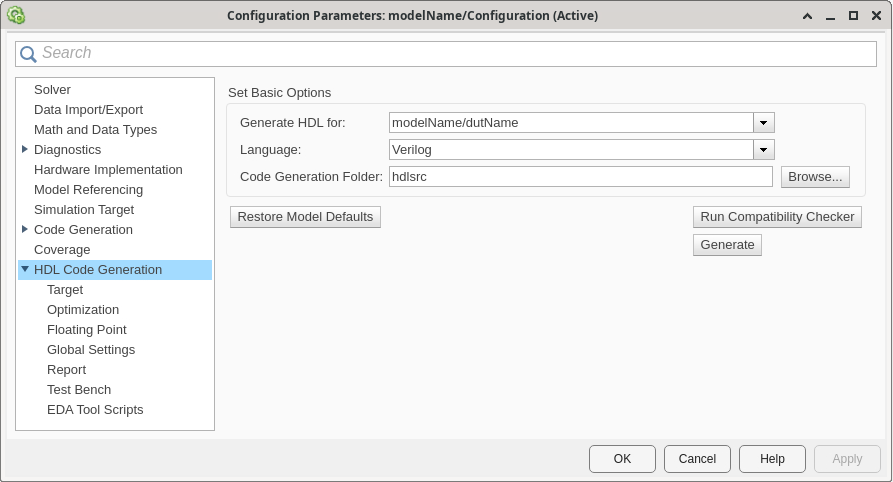
Open the Configuration Parameters dialog box by clicking Settings in the HDL Code tab.

In the HDL Code Generation pane, ensure that Language is set to Verilog. By default, HDL Coder generates the Verilog^® files in the hdlsrc folder. You can select an alternative location. If you make any changes, click Apply.

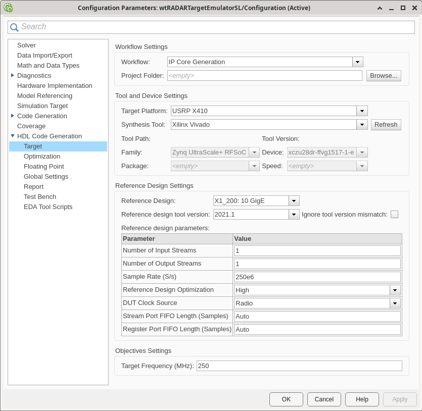
In the Target pane, configure these settings:

• Under Workflow Settings, select the IP Core Generation workflow. To set Project Folder, click Browse and select a target location for saving the generated project files. If you do not specify a project folder, the software saves the generated project files in the working directory.

• Under Tool and Device Settings, select your radio from the Target Platform list. This example uses a USRP X410 radio. If you are using a different radio, adjust the reference design parameters accordingly.

• Under Reference Design Settings, set Reference Design to the desired reference FPGA image for your design, based on how you set up your hardware. For a USRP X410 radio, you have one option: X1_200: 10GigE.

  Set the reference design parameters to these values:

  • Number of Input Streams — Set to 1 because the DUT is connected to one data input stream.

  • Number of Output Streams — Set to 1 because the DUT is connected to one data output stream.

  • Sample Rate (S/s) — Set to the maximum supported master clock rate (MCR) for the target device. This value is set by default. For an X410 radio, this value is 250e6. To determine which sample rates are available for your radio, see Determine Radio Device Capabilities.

  • Reference Design Optimization — Set to High. This is the maximum level of optimization level that maintains some debugging capability for exercising the design running on your radio. This optimization level reduces the resources associated with the reference design by:

    • Removing all resampling logic. Because the design uses an MCR as the sample rate, this logic is not required.

    • Removing all unused antennas. The reference design includes the antennas you select as DUT input or output connections in the Interface Mapping table, and an additional transmit and capture antenna for test and debug workflows. Any additional antenna connections are removed from the reference design.

  • DUT Clock Source — Set to Radio. When you select this setting, the DUT is clocked at the MCR used by the radio to achieve the specified sample rate. Alternatively, you can set this setting to Custom to set the DUT clock frequency to a user-defined value in the Target Frequency parameter under Objectives Settings.

  • Stream Port FIFO Length (Samples) — Set to Auto. This setting automatically calculates the buffer length for each DUT input and output data streaming port.

  • Register Port FIFO Length (Samples) — Set to Auto. This setting automatically calculates the buffer length for each DUT register port.

  Under Objectives Settings, since the DUT Clock Source is set to Radio, the Target Frequency is fixed at the highest supported MCR of the radio.

Click Apply.

In the Optimization pane, select Distributed pipelining.

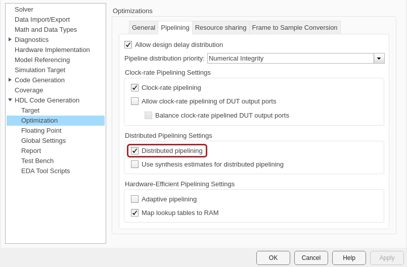
To apply these settings and close the Configuration Parameters window, click OK.

For more information, see Configure HDL Code Generation Settings.

Map Target Interfaces

In the HDL Code tab, click Target Interface to open the Interface Mapping table in the IP Core editor. To populate the table with your user logic, click the Reload IP core settings button: .

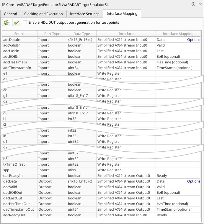
The Source, Port Type, and Data Type columns are populated based on the Simulink model. The Interface column automatically populates based on the port names in your model:

• The input register ports map to Write Register interfaces.

• The adcDataIn, adcValidIn, adcLastIn, adcEOBIn, adcHasTimeIn, adcTimestampIn, and adcReadyOut ports map to a Simplified AXI4-stream Input0 interface.

• The dacDataOut, dacValidOut, dacLastOut, dacEOBOut, dacHasTimeOut, dacTimestampOut, and dacReadyIn ports map to a Simplified AXI4-stream Output0 interface.

The Interface Mapping column is populated automatically based on the port names in the model.

To set the interface options for the streaming interfaces, open the Set Interface Options window by clicking Options in the far right of the table.

For the adcDataIn interface options, select a receive antenna as the source connection. The DUT receives input samples from this antenna on the radio. Set the stream buffer size to 32768, which is the default setting. The buffer size must be a power of two to ensure optimal use of the FPGA RAM resources. The buffer size is specified in terms of the number of samples, with each sample having a size of 8 bytes.

For the dacDataOut options, select a transmit antenna as the sink connection. The DUT sends output samples to this antenna on the radio for transmission.

When you have populated the table, validate the interface mapping by clicking the Validate IP core settings button: .

For more information, see Map Target Interfaces.

Generate and Load Bitstream

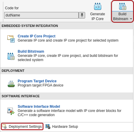
To generate a bitstream from the configured IP core, first open the deployment settings from the Build Bitstream button.

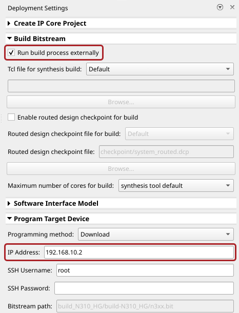
• Ensure that the Run build process externally option is selected. This setting is the default and it ensures that the bitstream build executes in an external shell, which allows you to continue using MATLAB while building the FPGA image.

• In the Program Target Device settings, set the IP address. The default is 192.168.10.2. If your radio has a different IP address, update this field with the correct value.

Click Build Bitstream to create a Vivado IP core project and build the bitstream. After the basic project checks complete, the Diagnostic Viewer displays a Build Bitstream Successful message along with warning messages. However, you must wait until the external shell displays a successful bitstream build before moving to the next step. Closing the external shell before this time terminates the build.

The bitstream for this project generates with the name n3xx.bit and is located in the build_N320_HG/build_N320_HG folder of the working directory after a successful bitstream build. If you are using a different radio, the name and location reflects your radio.

To load the bitstream onto the device now, click Program Target Device from the Build Bitstream button. Alternatively, you can load the bitstream later by using the programFPGA function in the generated host interface script.

For more information, see Generate Bitstream and Program FPGA.

Generate Host Interface Scripts

To generate MATLAB scripts that enable you to connect to and run your deployed design on your radio, in the HDL Code tab, click Host Interface Script. This step generates two scripts in your working directory based on the target interface mapping that you configured for your IP core.

• gs_wtRADARTargetEmulatorSL_interface.m — Host interface script that creates an fpga object for interfacing with your DUT running on the FPGA from MATLAB. The script contains code that connects to your hardware and programs the FPGA and code samples to get you started with running the algorithm on your radio. For more information, see Interface Script File.

• gs_wtRADARTargetEmulatorSL_setup.m — Setup function that configures the fpga object with the hardware interfaces and ports from your DUT algorithm. The function contains DUT port objects that have the port name, direction, data type, and interface mapping information, which it maps to the corresponding interfaces. For more information, see Setup Function File.

  Note

  The number of samples, specified in the FrameSize property, is set by default to 1e5. To change this value or the value of the Timeout property, manually edit the setup function.

Verify Radar Target Emulator Algorithm Using MATLAB

To verify the algorithm running on your radio, use this modified version of the host interface script to run a target scenario.

To test the target emulation algorithm on a single radio, the script follows these steps:

1. Set up and configure the radio with the generated bitstream and interfaces.

2. Configure additional radio antennas for transmit and capture from the host.

3. Configure the target emulation DUT with the default scenario parameters.

4. Schedule the transmission of a radar pulse train.

5. Schedule the streaming of IQ samples from the air into the onboard memory.

6. Plot the range-Doppler response for the samples received to the host.

Open Live Script

You can open this live script in MATLAB from the example working directory and use it interactively. In the Files panel, navigate to your example working directory and open VerifyRadarTargetEmulationAlgorithmUsingMATLABExample.m.

Set Up Radar Scenario

Customize the simulation for your radio hardware by editing the helperRadarTargetSimulationSetup function. Run the target simulator setup helper function with no input arguments to use the default parameters.

sim_in = helperRadarTargetSimulationSetup();

Select Radio

Call the radioConfigurations function. The function returns all available radio setup configurations that you saved using the Radio Setup wizard.

savedRadioConfigurations = radioConfigurations;

To update the menu with your saved radio setup configuration names, click Update. Then select the radio to use with this example.

savedRadioConfigurationNames = [string({savedRadioConfigurations.Name})];
radioConfig = savedRadioConfigurationNames(1) ;

Evaluate the transmit and receive antennas available on your radio device. You select transmit and capture antennas from the available options later in the script.

availableReceiveAntennas = hCaptureAntennas(radioConfig);
availableTransmitAntennas = hTransmitAntennas(radioConfig);

Create Radio Object

Use the radioConfigurations function to create a radio object.

radio = radioConfigurations(radioConfig);

Create usrp System Object

Create a usrp System object™ with the specified radio. This System object controls the radio hardware.

device = usrp(radio);

Program FPGA

If you have not yet programmed your device with the bitstream, select the program bitstream option. Update the code with your bitstream and hand-off information files. You can find these in the generated host interface script, gs_wtRADARTargetEmulator_interface. If your radio device is a USRP X310, you only require a bitstream file to program the FPGA.

programBitstream = false;
if(programBitstream)
     programFPGA(device, ...
         "build_X410_X1_200/build-X410_X1_200/x4xx.bit", ...    % replace with your .bit file
         "build_X410_X1_200/build/usrp_x410_fpga_X1_200.dts");  % replace with your .dts file
end

To configure the DUT interfaces according to the hand-off information file, use the describeFPGA function. Calling this function additionally sets the values for the SampleRate, DUTInputAntennas, and DUTOutputAntennas properties based on the selections you made in Simulink.

% replace with your .mat handoff file
describeFPGA(device,"wtRADARTargetEmulatorSL_wthandoffinfo.mat"); 

Configure Device

Configure your usrp System object to loop back the waveform through the target emulator. You can loop back over the air or directly on the FPGA.

Set the sample rate according to the simulation setup defined in the helperRadarTargetSimulationSetup function.

device.SampleRate = sim_in.Fs;

Set the LoopbackMode property to FPGA to loop back each transmit antenna to an associated receive antenna on the FPGA. Alternatively, you can select Disabled to transmit and receive data over the air. FPGA loopback is not available on radios that have no transmit antennas.

device.LoopbackMode = "FPGA";

Because the bitstream was generated with the Reference Design Optimization parameter set to High, the radio antennas connected to the DUT are fixed to the options you configured in the Interface Mapping table in Simulink. To use FPGA loopback, your DUT must be configured with an input and output antenna connection that is a valid loopback antenna pair. For details, refer to the table in the LoopbackMode property description.

Specify a transmit antenna and a capture antenna to exercise the target emulation DUT from MATLAB. Because the bitstream is generated with the Reference Design Optimization parameter set to High, there is a single transmit and capture antenna available.

% MATLAB IO Antennas
device.TransmitAntennas = availableTransmitAntennas(1);
device.CaptureAntennas = availableReceiveAntennas(2);

Specify the center frequency and gain for the selected transmit and receive antennas. To loop back over the air, ensure the transmit and receive center frequencies are equal. If an FPGA loop back has been selected, these properties have no effect.

To isolate the two pairs of antennas either use loopback cables or separate the antennas in frequency by specifying multiple center frequency values. If you are using an USRP N310 radio, specifying multiple center frequencies may not be possible.

device.ReceiveCenterFrequency = [2.4e9,2.8e9];
device.TransmitCenterFrequency = device.ReceiveCenterFrequency(2:-1:1);

Specify the desired RF gain for the target emulator input and output. The output gain should be specified as a reference corresponding to the maximum output power of the target emulator in the initial state.

targetEmulatorInputRadioGain = 30; 
targetEmulatorOutputRadioGainReference = 30;

Specify the radio gains for the MATLAB transmit and capture antennas. Set the value according to your RF setup and hardware.

mlCaptureRadioGain = 30; 
mlTransmitRadioGain = 30;

Set the radio gain values for each antenna using the usrp System object.

device.ReceiveRadioGain = [targetEmulatorInputRadioGain,mlCaptureRadioGain];
device.TransmitRadioGain = [targetEmulatorOutputRadioGainReference,mlTransmitRadioGain];

Create and Setup FPGA Object

To interface with the ports on the DUT you designed in Simulink, create an fpga object with the device System object.

dut = fpga(device);

Set up the fpga object using the setup function you generated in the Simulink toolstrip workflow.

gs_wtRADARTargetEmulatorSL_setup(dut);

Optimize Round-trip Latency

To optimize the round-trip latency of the target emulator, tune the samples per AXI-4 streaming packet and the overall scheduled re-transmission time offset.

The samples per packet (SPP) input defines the number of valid samples between assertions of the last signal. If the SPP input is zero, which is the default value of the register on the hardware, the SPP used is 256. By specifying a lower value the packet latency will be reduced, and as a tradeoff the overhead of the streaming connection will increase which reduces maximum throughput. If the SPP is set too low overflows will occur. The optimal value is dependent on the specific hardware setup.

The txTimeOffset input sets the scheduled re-transmission time as an offset from the received timestamp. If the reTxOffset is set to zero, the transmission is scheduled as soon as possible. Specifying a non-zero value for reTxOffset from MATLAB allows for precise sample-level control of the round-trip latency inside the FPGA. If the reTxOffset is too short the burst may arrive late at the radio front end. If the txTimeOffset is longer than the available buffers then overflows will occur due to backpressure. The optimal value varies depending on the specific hardware setup and the specified SPP.

These values, SPP equal to 100 and reTxOffset set to 258, are tuned on a USRP X410 and USRP N320 radio. You may need to tune these values for other radio hardware. In general, SPP equal to 256 and reTxOffset equal to 258 is a reliable configuration.

device.SamplesPerPacket = 100; 
reTxOffset = 258;

Setup USRP Object

To establish a connection with the radio hardware, call setup on the device System object.

setup(device);

Reconnecting to radio. Radio time will be reset.

Set Initial Target Emulator State

After connecting to the radio, configure the register ports on the target emulator algorithm using the writePort function according to the default target scenario state in the helperRadarTargetSimulationSetup function.

Specify the front end delay so that it can be accounted for in the simulation. When using FPGA loopback mode, set this value to zero. If this is not accounted for when you transmit and receive the data over the air, there will be a small shift in the estimated ranges. Calibrate the additional delay for your radio front end by doing a timed loopback.

calibratedFrontEndDelay = 0;

Update the register ports of the target emulator.

% Convert to increment and sample delay
TargetInc = sim_in.TargetDoppler.*(2^sim_in.TargetEmulator_NCO_accum_wl/sim_in.Fs); % DopFreq to inc
TargetDelaySamples = nearest(abs(sim_in.TargetDelay).*sim_in.Fs - reTxOffset - calibratedFrontEndDelay); % Time to samples

writePort(dut, "spp", device.SamplesPerPacket); % Match the SPP of the radio input
writePort(dut, "txTimeOffset", reTxOffset); % Re-transmit at a known time offset
for target = 1:length(sim_in.TargetEnabled)
    writePort(dut, "e"+string(target), sim_in.TargetEnabled(target));
    if sim_in.TargetEnabled(target) % If enabled, write delay, inc and gain
        writePort(dut, "d"+string(target), TargetDelaySamples(target)); % Delay relative to the expected minimum latency
        writePort(dut, "i"+string(target), TargetInc(target));
        writePort(dut, "g"+string(target), sim_in.TargetGain(target));
    end
end

Configure Transmit Waveform

Format the transmit waveform pulse train according to the slow time dimension length. Then scale as a 16 bit integer.

txPulseTrain = repmat( ...
    [sim_in.txSignal; zeros(sim_in.pulsePeriodSamples-length(sim_in.txSignal),1)], ...
    sim_in.VelDimLen, 1)*double(intmax('int16'));
captureLength = length(txPulseTrain);

Specify a scheduling offset. This is the number of seconds in the future the transmit and receive operations will start. The offset must be long enough to account the loading of the transmit waveform into the PL DDR buffer before the start of the transmission.

scheduleTimeOffset = 1;

Configure Detection

Create a phased.RangeDopplerResponse (Phased Array System Toolbox) object to analyze the received responses.

rdResponse = phased.RangeDopplerResponse(...
    DopplerFFTLengthSource='Property', ...
    DopplerFFTLength=sim_in.VelDimLen, ...
    PRFSource='Property',PRF=sim_in.PRF,...
    SampleRate=sim_in.Fs, ...
    DopplerOutput="Speed", ...
    OperatingFrequency=sim_in.Fc);

Create a 2D constant false alarm rate (CFAR) object for detection generation. For optimal results, tune the parameters for your radio and setup.

cfar = phased.CFARDetector2D(GuardBandSize=[25 1], ...
    TrainingBandSize=[10 1],ProbabilityFalseAlarm=1e-4);

Verify DUT

Simulate the default scenario to verify the behavior is as expected.

First, schedule the transmit and receive operations to begin at the specified time offset.

currentRadioTime = getRadioTime(radio);
scheduledTime = currentRadioTime + scheduleTimeOffset;

Use the transmit function to schedule a single-shot transmission at the specified time.

transmit(device,txPulseTrain,"once",StartTime=scheduledTime);
device(captureLength,StartTime=scheduledTime,Background=false); 

Use the capture function to retrieve the captured samples from the PL DDR buffer.

[out.DataOut,nSamps] = capture(device,captureLength); 
out.ValidOut = true(1,nSamps);

Visualize the received RF data using the helperVisualizeRadarTargetSimulation function. The helper function plots the range-Doppler response and overlays both the 2D CFAR detection and expected target range-Doppler coordinates.

fig = figure;
ax = axes(fig);
helperVisualizeRadarTargetSimulation(out,sim_in,rdResponse,cfar,0,ax);

Release Hardware Resources

Stop the transmission and release the hardware resources.

release(dut);
release(device);

Next Steps

To use your deployed design to simulate a full pulse radar scenario, use the Pulse Radar Scenario Using Target Emulator on NI USRP Radio example. This example enables you to customize the scenario and simulate all frames.

Use Target Emulator in Deployment Scenarios

You can use the deployed design to test various radar target emulation scenarios using real world signals. These examples provide host interface scripts that enable you to exercise and verify the deployed design in different deployment scenarios. For more information, see Radar Target Emulation Applications Overview.

Example	Deployment Test Scenario
Pulse Radar Scenario Using Target Emulator on NI USRP Radio	Run a pulse radar scenario on an NI USRP radio with the target emulation algorithm deployed on the FPGA. Use the same radio to transmit a linear FM radar pulse train, then capture and plot the emulated target range-Doppler response in MATLAB.
Real Time Target Emulation on NI USRP Radio	Run a pulse radar scenario on an NI USRP radio with the target emulation algorithm deployed on the FPGA, running continuously. Use a second NI USRP radio to transmit a linear FM radar pulse train, then capture and plot the emulated target range-Doppler response in MATLAB.
Integrated Sensing and Communication Using 6G Waveform on NI USRP Radio	Generate a 6G waveform to track a moving object in an integrated sensing and communications (ISAC) scenario. Use the same radio to transmit the generated waveform, then capture and plot the emulated target range-Doppler response in MATLAB.