Resultados de
In case you haven't come across it yet, @Gareth created a Jokes toolbox to get MATLAB to tell you a joke.
Dear MATLAB contest enthusiasts,
In the 2023 MATLAB Mini Hack Contest, Tim Marston captivated everyone with his incredible animations, showcasing both creativity and skill, ultimately earning him the 1st prize.
We had the pleasure of interviewing Tim to delve into his inspiring story. You can read the full interview on MathWorks Blogs: Community Q&A – Tim Marston.
Last question: Are you ready for this year’s Mini Hack contest?
As far as I know, starting from MATLAB R2024b, the documentation is defaulted to be accessed online. However, the problem is that every time I open the official online documentation through my browser, it defaults or forcibly redirects to the documentation hosted site for my current geographic location, often with multiple pop-up reminders, which is very annoying!
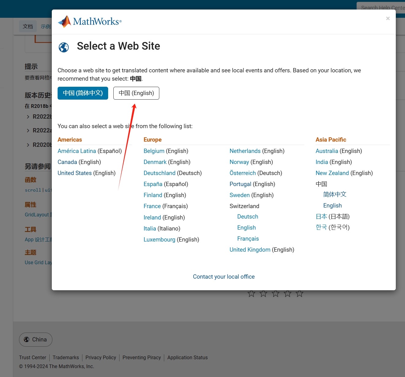
Suggestion: Could there be an option to set preferences linked to my personal account so that the documentation defaults to my chosen language preference without having to deal with “forced reminders” or “forced redirection” based on my geographic location? I prefer reading the English documentation, but the website automatically redirects me to the Chinese documentation due to my geolocation, which is quite frustrating!
----------------2024.12.13 update-----------------
Although the above issue was resolved by technical support, subsequent redirects are still causing severe delays...
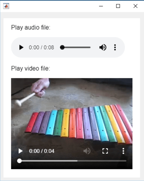
In the past two years, MATHWORKS has updated the image viewer and audio viewer, giving them a more modern interface with features like play, pause, fast forward, and some interactive tools that are more commonly found in typical third-party players. However, the video player has not seen any updates. For instance, the Video Viewer or vision.VideoPlayer could benefit from a more modern player interface. Perhaps I haven't found a suitable built-in player yet. It would be great if there were support for custom image processing and audio processing algorithms that could be played in a more modern interface in real time.
Additionally, I found it quite challenging to develop a modern video player from scratch in App Designer.(If there's a video component for that that would be great)
-----------------------------------------------------------------------------------------------------------------
BTW,the following picture shows the built-in function uihtml function showing a more modern playback interface with controls for play, pause and so on. But can not add real-time image processing algorithms within it.
isequaln exists to return true when NaN==NaN.
unique treats NaN==NaN as false (as it should) requiring NaN to be replaced if NaN is not considered unique in a particular application. In my application, I am checking uniqueness of table rows using [table_unique,index_unique]=unique(table,"rows","sorted") and would prefer to keep NaN as NaN or missing in table_unique without the overhead of replacing it with a dummy value then replacing it again. Dummy values also have the risk of matching existing values in the table, requiring first finding a dummy value that is not in the table.
uniquen (similar to isequaln) would be more eloquent.
Please point out if I am missing something!
Hi All,
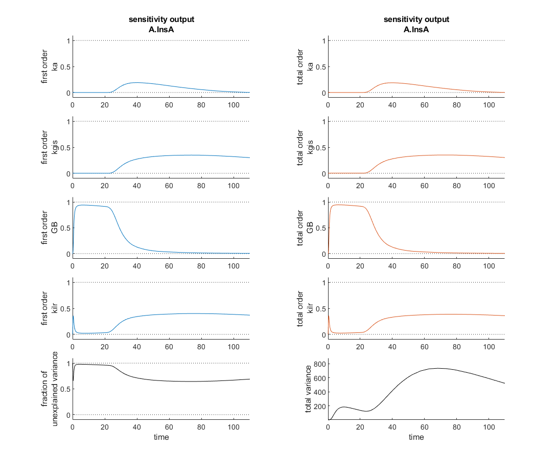
I'm currently verifying a global sensitivity analysis done in SimBiology and I'm a touch confused. This analysis was run with every parameter and compartment volume in the model. To my understanding the fraction of unexplained variance is 1 - the sum of the first order variances, therefore if the model dynamics are dominated by interparameter effects you might see a higher fraction of unexplained variance. In this analysis however, as the attached figure shows (with input at t=20 minutes), the most sensitive four parameters seem to sum, in first order sensitivities to roughly one at each time point and the total order sensitivies appear nearly identical. So how is the fraction of unexplained variance near one?
Thank you for your help!
Imagine that the earth is a perfect sphere with a radius of 6371000 meters and there is a rope tightly wrapped around the equator. With one line of MATLAB code determine how much the rope will be lifted above the surface if you cut it and insert a 1 meter segment of rope into it (and then expand the whole rope back into a circle again, of course).
hello i found the following tools helpful to write matlab programs. copilot.microsoft.com chatgpt.com/gpts gemini.google.com and ai.meta.com. thanks a lot and best wishes.
Check out the LLMs with MATLAB project on File Exchange to access Large Language Models from MATLAB.
Along with the latest support for GPT-4o mini, you can use LLMs with MATLAB to generate images, categorize data, and provide semantic analyis.
Something that had bothered me ever since I became an FEA analyst (2012) was the apparent inability of the "camera" in Matlab's 3D plot to function like the "cameras" in CAD/CAE packages.
For instance, load the ForearmLink.stl model that ships with the PDE Toolbox in Matlab and ParaView and try rotating the model.
clear
close all
gm = importGeometry( "ForearmLink.stl" );
pdegplot(gm)
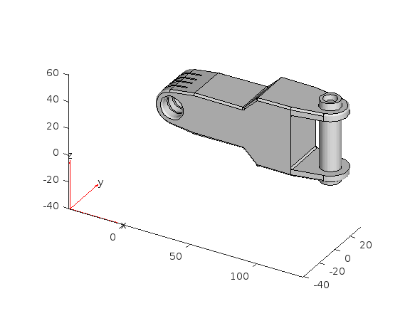
Things to observe:
- Note that I cant seem to rotate continuously around the x-axis. It appears to only support rotations from [0, 360] as opposed to [-inf, inf]. So, for example, if I'm looking in the Y+ direction and rotate around X so that I'm looking at the Z- direction, and then want to look in the Y- direction, I can't simply keep rotating around the X axis... instead have to rotate 180 degrees around the Z axis and then around the X axis. I'm not aware of any data visualization applications (e.g., ParaView, VisIt, EnSight) or CAD/CAE tools with such an interaction.
- Note that at the 50 second mark, I set a view in ParaView: looking in the [X-, Y-, Z-] direction with Y+ up. Try as I might in Matlab, I'm unable to achieve that same view perspective.
Today I discovered that if one turns on the Camera Toolbar from the View menubar, then clicks the Orbit Camera icon, then the No Principal Axis icon:
That then it acts in the manner I've long desired. Oh, and also, for the interested, it is programmatically available: https://www.mathworks.com/help/matlab/ref/cameratoolbar.html
I might humbly propose this mode either be made more discoverable, similar to the little interaction widgets that pop up in figures:
Or maybe use the middle-mouse button to temporarily use this mode (a mouse setting in, e.g., Abaqus/CAE).
I've noticed is that the highly rated fonts for coding (e.g. Fira Code, Inconsolata, etc.) seem to overlook one issue that is key for coding in Matlab. While these fonts make 0 and O, as well as the 1 and l easily distinguishable, the brackets are not. Quite often the curly bracket looks similar to the curved bracket, which can lead to mistakes when coding or reviewing code.
So I was thinking: Could Mathworks put together a team to review good programming fonts, and come up with their own custom font designed specifically and optimized for Matlab syntax?
An option for 10th degree polynomials but no weighted linear least squares. Seriously? Jesse
What do you think about the NVIDIA's achivement of becoming the top giant of manufacturing chips, especially for AI world?

Hi to everyone!
To simplify the explanation and the problem, I simulated the kinetics of an irreversible first-order reaction, A -> B. I implemented it in two independent compartments, R and P. I simulated the effect of a dilution in R by doubling at t= 0,1 the R volume. I programmed in P that, at t = 0.1, the instantaneous concentration of A and B would be reduced by half. I am sending an attach with the implementation of these simulations in the Simbiology interface.
When the simulations of the two compartments are plotted, it can be seen that the responses are not equal. That is, from t = 0.1 s, the reaction follow an exponential function in R with half of the initial amplitude and half of the initial value of k1. That is, the relaxation time is doubled. Meanwhile, in P, from t = 0.1, the reaction follows exponential kinetics with half the amplitude value but maintaining the initial value of k = 10. Without a doubt, the correct simulation is the latter (compartment P) where only the effect is observed in the amplitude and not in the relaxation time. Could you tell me what the error is that makes these kinetics that should be equal not be?
Thank you in advance!
Luis B.
Hi All,
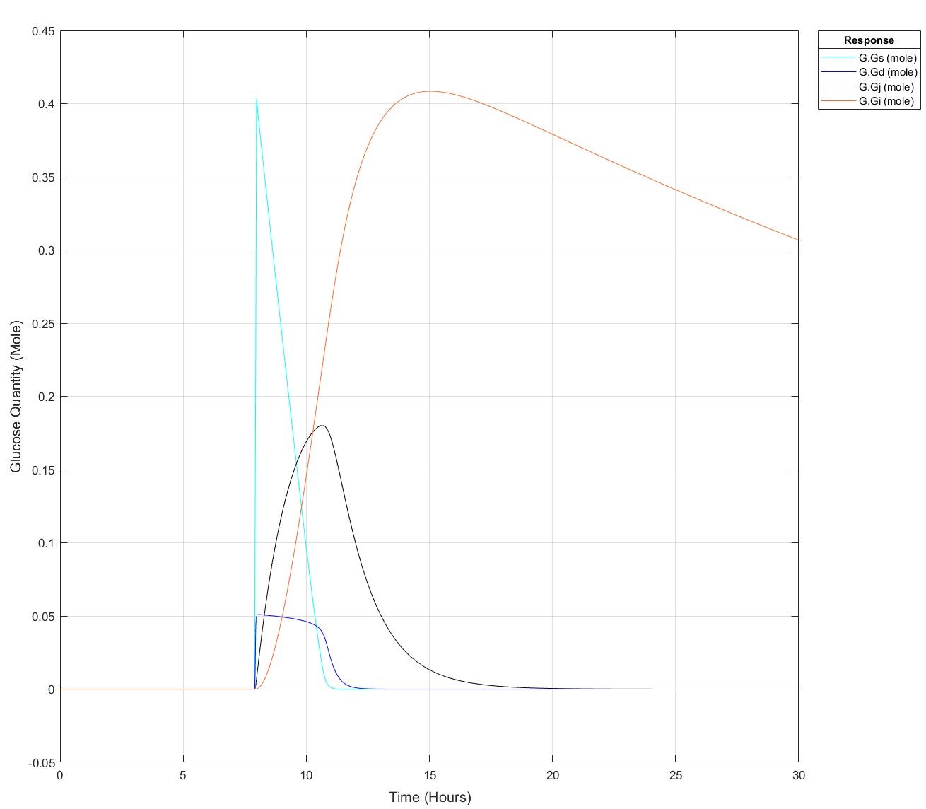
I've been producing a QSP model of glucose homeostasis for a while now for my PhD project, recently I've been able to expand it to larger time series, i.e. 2 days of data rather than a singular injection or a singular meal. My problem is as follows: If I put 75g of glucose into my stomach glucose species any later than (exactly) 8.5 hours I get an integration tolerance error. Curiosly, I can put 25g of glucose in at any time up to 15.9 hours, then any later an error. I have disabled all connections to my glucose absorption chain, i.e. stomach -> duodenum -> jenenum -> ileum -> removal, to isolate the cause of this. I had initially thought it may be because I mechanistically model liver glycogen and that does deplete over time, but I've tested enough to show that that does nothing. My next test is to isolate the glucose absorption chain into a seperate model and see if the issue persists but I'm completely baffled!
These are the equations, to my eye there's no reason why there would be such a sharp glucose quantity/time dependence, they all begin at a value of 0:
d(Gs)/dt = -(kw*(1-Gd^14/(Igd^14+Gd^14))*Gs) #Stomach glucose
d(Gd)/dt = (kw*(1-Gd^14/(Igd^14+Gd^14))*Gs) - (kdj*Gd) #Duodenal Glucose
d(Gj)/dt = (kdj*Gd) - (kji*Gj) #Jejunal Glucose
d(Gi)/dt = (kji*Gj) - (kic*Gi) #Ileal Glucose
(The sigmoidicity of gastric emptying slowing term (^14) was parameterised off of paracetamol absorption data and appears to be correct!)
Thank you for your help, best regards,
Dan
Pre-Edit: I changed the run time to 30 hours and now I can't use the 75g input any later than 7.9 hours not 8.5 hours anymore!
Edit: This is how it appears at all times prior to it failing for 75g:
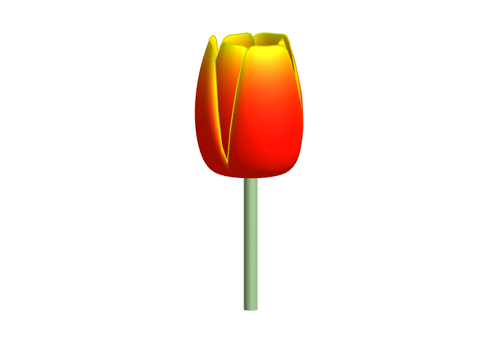
Spring is here in Natick and the tulips are blooming! While tulips appear only briefly here in Massachusetts, they provide a lot of bright and diverse colors and shapes. To celebrate this cheerful flower, here's some code to create your own tulip!
One of the starter prompts is about rolling two six-sided dice and plot the results. As a hobby, I create my own board games. I was able to use the dice rolling prompt to show how a simple roll and move game would work. That was a great surprise!
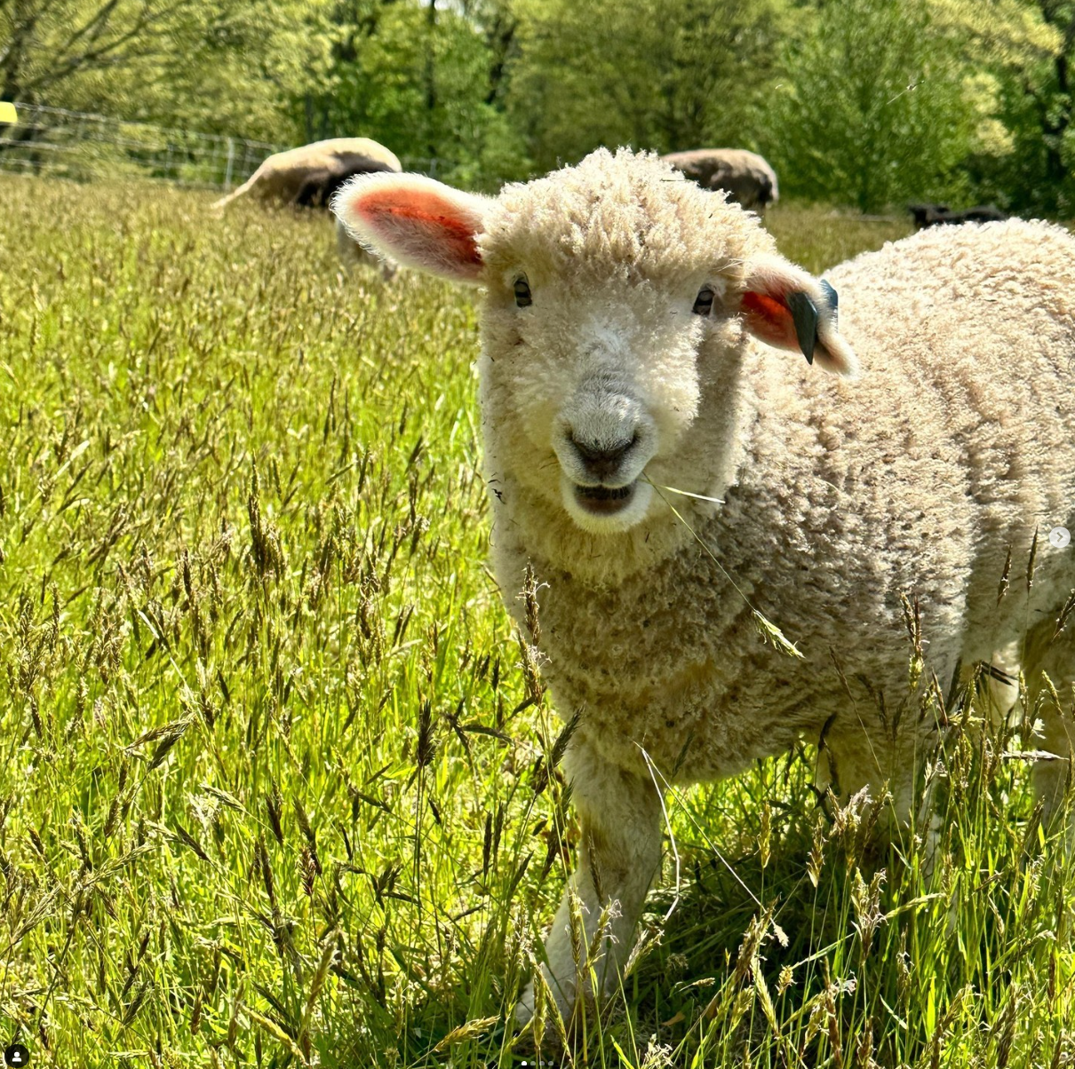
Drumlin Farm has welcomed MATLAMB, named in honor of MathWorks, among ten adorable new lambs this season!
I found this plot of words said by different characters on the US version of The Office sitcom. There's a sparkline for each character from pilot to finale episode.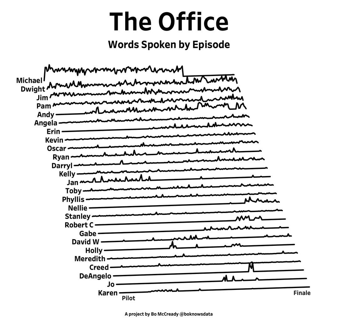
A high school student called for help with this physics problem:
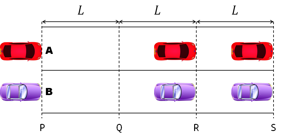
- Car A moves with constant velocity v.
- Car B starts to move when Car A passes through the point P.
- Car B undergoes...
- uniform acc. motion from P to Q.
- uniform velocity motion from Q to R.
- uniform acc. motion from R to S.
- Car A and B pass through the point R simultaneously.
- Car A and B arrive at the point S simultaneously.
Q1. When car A passes the point Q, which is moving faster?
Q2. Solve the time duration for car B to move from P to Q using L and v.
Q3. Magnitude of acc. of car B from P to Q, and from R to S: which is bigger?
Well, it can be solved with a series of tedious equations. But... how about this?
Code below:
%% get images and prepare stuffs
figure(WindowStyle="docked"),
ax1 = subplot(2,1,1);
hold on, box on
ax1.XTick = [];
ax1.YTick = [];
A = plot(0, 1, 'ro', MarkerSize=10, MarkerFaceColor='r');
B = plot(0, 0, 'bo', MarkerSize=10, MarkerFaceColor='b');
[carA, ~, alphaA] = imread('https://cdn.pixabay.com/photo/2013/07/12/11/58/car-145008_960_720.png');
[carB, ~, alphaB] = imread('https://cdn.pixabay.com/photo/2014/04/03/10/54/car-311712_960_720.png');
carA = imrotate(imresize(carA, 0.1), -90);
carB = imrotate(imresize(carB, 0.1), 180);
alphaA = imrotate(imresize(alphaA, 0.1), -90);
alphaB = imrotate(imresize(alphaB, 0.1), 180);
carA = imagesc(carA, AlphaData=alphaA, XData=[-0.1, 0.1], YData=[0.9, 1.1]);
carB = imagesc(carB, AlphaData=alphaB, XData=[-0.1, 0.1], YData=[-0.1, 0.1]);
txtA = text(0, 0.85, 'A', FontSize=12);
txtB = text(0, 0.17, 'B', FontSize=12);
yline(1, 'r--')
yline(0, 'b--')
xline(1, 'k--')
xline(2, 'k--')
text(1, -0.2, 'Q', FontSize=20, HorizontalAlignment='center')
text(2, -0.2, 'R', FontSize=20, HorizontalAlignment='center')
% legend('A', 'B') % this make the animation slow. why?
xlim([0, 3])
ylim([-.3, 1.3])
%% axes2: plots velocity graph
ax2 = subplot(2,1,2);
box on, hold on
xlabel('t'), ylabel('v')
vA = plot(0, 1, 'r.-');
vB = plot(0, 0, 'b.-');
xline(1, 'k--')
xline(2, 'k--')
xlim([0, 3])
ylim([-.3, 1.8])
p1 = patch([0, 0, 0, 0], [0, 1, 1, 0], [248, 209, 188]/255, ...
EdgeColor = 'none', ...
FaceAlpha = 0.3);
%% solution
v = 1; % car A moves with constant speed.
L = 1; % distances of P-Q, Q-R, R-S
% acc. of car B for three intervals
a(1) = 9*v^2/8/L;
a(2) = 0;
a(3) = -1;
t_BatQ = sqrt(2*L/a(1)); % time when car B arrives at Q
v_B2 = a(1) * t_BatQ; % speed of car B between Q-R
%% patches for velocity graph
p2 = patch([t_BatQ, t_BatQ, t_BatQ, t_BatQ], [1, 1, v_B2, v_B2], ...
[248, 209, 188]/255, ...
EdgeColor = 'none', ...
FaceAlpha = 0.3);
p3 = patch([2, 2, 2, 2], [1, v_B2, v_B2, 1], [194, 234, 179]/255, ...
EdgeColor = 'none', ...
FaceAlpha = 0.3);
%% animation
tt = linspace(0, 3, 2000);
for t = tt
A.XData = v * t;
vA.XData = [vA.XData, t];
vA.YData = [vA.YData, 1];
if t < t_BatQ
B.XData = 1/2 * a(1) * t^2;
vB.XData = [vB.XData, t];
vB.YData = [vB.YData, a(1) * t];
p1.XData = [0, t, t, 0];
p1.YData = [0, vB.YData(end), 1, 1];
elseif t >= t_BatQ && t < 2
B.XData = L + (t - t_BatQ) * v_B2;
vB.XData = [vB.XData, t];
vB.YData = [vB.YData, v_B2];
p2.XData = [t_BatQ, t, t, t_BatQ];
p2.YData = [1, 1, vB.YData(end), vB.YData(end)];
else
B.XData = 2*L + v_B2 * (t - 2) + 1/2 * a(3) * (t-2)^2;
vB.XData = [vB.XData, t];
vB.YData = [vB.YData, v_B2 + a(3) * (t - 2)];
p3.XData = [2, t, t, 2];
p3.YData = [1, 1, vB.YData(end), v_B2];
end
txtA.Position(1) = A.XData(end);
txtB.Position(1) = B.XData(end);
carA.XData = A.XData(end) + [-.1, .1];
carB.XData = B.XData(end) + [-.1, .1];
drawnow
end