i-vector Score Normalization
An i-vector system outputs a raw score specific to the data and parameters used to develop the system. This makes interpreting the score and finding a consistent decision threshold for verification tasks difficult.
To address these difficulties, researchers developed score normalization and score calibration techniques.
In score normalization, raw scores are normalized in relation to an 'imposter cohort'. Score normalization occurs before evaluating the detection error tradeoff and can improve the accuracy of a system and its ability to adapt to new data.
In score calibration, raw scores are mapped to probabilities, which are used to better understand the system's confidence in decisions.
In this example, you apply score normalization to an i-vector system. To learn about score calibration, see i-vector Score Calibration.
For example purposes, you use cosine similarity scoring (CSS) throughout this example. Probabilistic linear discriminant analysis (PLDA) scoring is also improved by normalization, although less dramatically.
Download i-vector System and Data Set
To download a pretrained i-vector system suitable for speaker recognition, call speakerRecognition. The ivectorSystem returned was trained on the LibriSpeech data set, which consists of English-language 16 kHz recordings.
ivs = speakerRecognition();
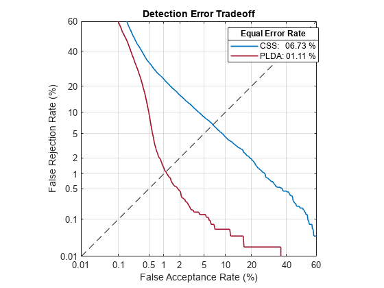
The pretrained i-vector system achieves an equal error rate (EER) around 6.73% using CSS on the LibriSpeech test set. The EER achieved using PLDA is considerably better. However, because CSS is simpler, for the purposes of this example you investigate CSS only.
detectionErrorTradeoff(ivs)
The error rate on the LibriSpeech test set, and the accompanying default decision threshold for speaker verification, do not extend well to unseen data. To confirm this, download the PTDB-TUG [3] data set. The supporting function, loadDataset, downloads the data set and then resamples it from 48 kHz to 16 kHz, which is the sample rate that the i-vector system was trained on. The loadDataset function returns four audioDatastore objects:
adsEnroll- Contains files to enroll speakers into i-vector system.adsTest- Contains files to spot-check performance of the i-vector system.adsDET- Contains a large set of files to analyze the detection error tradeoff of the i-vector system.adsImposter - Contains a set of speakers not included in the other datastores. This set is used for score normalization.
targetSampleRate = ivs.SampleRate;
[adsEnroll,adsTest,adsDET,adsImposter] = loadDataset(targetSampleRate);
Enroll speakers from the enrollment dataset. When you enroll speakers, an i-vector template is created for each unique speaker label.
enroll(ivs,adsEnroll,adsEnroll.Labels)
Extracting i-vectors ...done.
Enrolling i-vectors ...................done.
Enrollment complete.
enrolledLabels = categorical(ivs.EnrolledLabels.Properties.RowNames);
Spot-check the false rejection rate (FRR) and the false acceptance rate (FAR) using the verify object function. The verify object function scores the i-vector derived from the audio input against the i-vector template corresponding to the specified label. The function then compares the score to a decision threshold and either accepts or rejects the proposition that the audio input belongs to the specified speaker label. The default decision threshold corresponds to the equal error rate (EER) determined the last time the detection error tradeoff was evaluated.
FA = 0;
FR = 0;
reset(adsTest)
numToSpotCheck = 50;
for ii = 1:numToSpotCheck
    [audioIn,fileInfo] = read(adsTest);
    targetLabel = fileInfo.Label;

    FR = FR + ~verify(ivs,audioIn,targetLabel,"css");

    nontargetIdx = find(~ismember(enrolledLabels,targetLabel));
    nontargetLabel = enrolledLabels(nontargetIdx(randperm(numel(nontargetIdx),1)));

    FA = FA + verify(ivs,audioIn,nontargetLabel,"css");
end
FRR = FR./numToSpotCheck;
FAR = FA./numToSpotCheck;
disp(["False Rejection Rate = " + round(100*FRR,2) + " (%)"; ...
    "False Acceptance Rate = " + round(100*FAR,2) + " (%)"])
    "False Rejection Rate = 0 (%)"
    "False Acceptance Rate = 38 (%)"
The performance on this new dataset does not match performance reported when training and evaluating the i-vector system on the LibriSpeech data set. Also, the default decision threshold on the LibriSpeech data set does not correspond to the equal error rate on the PTDB-TUG data set.
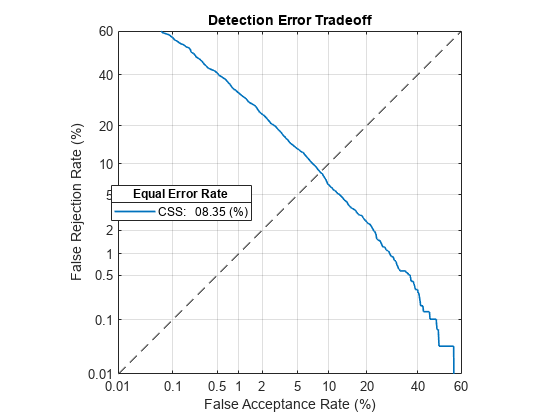
To better evaluate the system's performance, and to choose a new decision threshold, call detectionErrorTradeoff again. This time call detectionErrorTradeoff with new evaluation data that is more suited to the target application. The evaluation data should be as close as possible to the data that your deployed system encounters in terms of vocabulary, prosody, signal duration, noise level, noise type, accents, channel characteristics, and so on.
detectionErrorTradeoff(ivs,adsDET,adsDET.Labels,Scorer="css")Extracting i-vectors ...done. Scoring i-vector pairs ...done. Detection error tradeoff evaluation complete.
Spot-check the FAR and FRR of the updated system. The FAR and FRR are now reasonably close to the EER reported in the detection error tradeoff analysis. Note that calling detectionErrorTradeoff does not modify the i-vector extraction or scoring, only the default decision threshold for speaker verification. In the following sections, you enhance an i-vector system to perform score normalization. Score normalization helps an i-vector system extend to new datasets without the need to reevaluate the detection error tradeoff. Score normalization also helps bridge the performance gap between training a system and deploying it.
FA = 0;
FR = 0;
reset(adsTest)
for ii = 1:numToSpotCheck
    [audioIn,fileInfo] = read(adsTest);
    trueLabel = fileInfo.Label;

    FR = FR + ~verify(ivs,audioIn,trueLabel,"css");

    imposterIdx = find(~ismember(enrolledLabels,trueLabel));
    imposter = enrolledLabels(imposterIdx(randperm(numel(imposterIdx),1)));

    FA = FA + verify(ivs,audioIn,imposter,"css");
end
FRR = FR./numToSpotCheck;
FAR = FA./numToSpotCheck;
disp(["False Rejection Rate = " + round(100*FRR,2) + " (%)"; ...
    "False Acceptance Rate = " + round(100*FAR,2) + " (%)"])
    "False Rejection Rate = 4 (%)"
    "False Acceptance Rate = 8 (%)"
Score Normalization
Score normalization is a common approach to make target and non-target score distributions across speakers more similar. This enables a system to set a decision threshold that is closer to optimal for more speakers. In this example, you explore adaptive symmetric normalization variant 1 (S-norm1) [1].
To motivate score normalization, first inspect the target and non-target score distributions for two enrolled labels against the same test cohort.
Isolate two template i-vectors corresponding to two speakers.
enrolledIvecs = cat(2,ivs.EnrolledLabels.ivector{1},ivs.EnrolledLabels.ivector{9});
label_e = categorical([ivs.EnrolledLabels.Properties.RowNames(1),ivs.EnrolledLabels.Properties.RowNames(9)]);
Extract i-vectors from the test set. The test set labels overlap with the enrolled labels.
testIvecs = ivector(ivs,adsTest);
label_t = adsTest.Labels;
Create indexing vectors to keep track of which test i-vectors correspond to which enrolled label. In the targets matrix, the columns correspond to the enrolled speakers, and the rows correspond to the test files. If the test label corresponds to the enrolled label, the value in the matrix is true, otherwise, the value is false.
targets = [ismember(label_t,label_e(1)),ismember(label_t,label_e(2))];
Score the template i-vectors against the target and non-target i-vectors. The supporting function, scoreTargets, scores all combinations of the enrolled i-vectors against the test i-vectors and returns the scores separated into target scores (when the test and enroll labels are the same) and non-target scores (when the test and enroll labels are different).
[targetScores,nontargetScores] = scoreTargets(enrolledIvecs,testIvecs,targets);
Use the supporting function, plotScoreDistributions, to display the target and non-target scores for each of the enrolled speakers. Note that the equal error rate (where the target and non-target distributions cross) is different for the two speakers. That is, assuming the equal error rate is the goal of the system, a single decision threshold cannot capture the equal error rate for both speakers.
plotScoreDistributions(targetScores,nontargetScores,Analyze="label")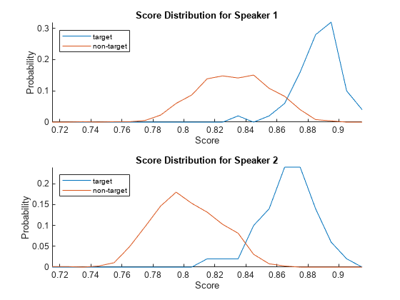
Analyze the score distributions using an EER plot. EER plots reveal the relationship between a decision threshold and the probability of a false alarm or false rejection and are often analyzed to determine a decision threshold.
plotEER(targetScores,nontargetScores,Analyze="label")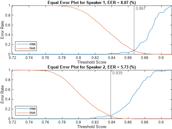
Analyze Score Normalization on Two Speakers
In this example, you use adaptive symmetric normalization variant 1 (S-norm1) [1]. S-norm1 computes an average of normalized scores from Z-norm (zero score normalization) and T-norm (test score normalization).
where
is the raw score based on the enrollment and test i-vectors.
is the set of the top-scoring imposter cohort with enrolled i-vector, .
is the set of the top-scoring imposter cohort with test i-vector, .
, is the set of cohort scores formed by scoring enrollment utterance with the top files from imposter cohort .
, is the set of the top scores between an enrolled i-vector and imposter i-vectors.
, is the set of the top scores between a test i-vector and imposter i-vectors.
and are the mean and standard deviation of .
To begin, extract i-vectors from the imposter cohort ().
imposterIvecs = ivector(ivs,adsImposter);
Score the enrolled i-vectors against the imposter cohort () and then isolate only the K best scores (). [1] suggests using the top 200-500 scoring files to create a speaker-dependent cohort. Finally, calculate the mean () and standard deviation ().
topK =400; imposterScores = sort(cosineSimilarityScore(enrolledIvecs,imposterIvecs),"descend"); imposterScores = imposterScores(1:min(topK,size(imposterScores,1)),:); mu_e = mean(imposterScores,1); std_e = std(imposterScores,[],1);
Calculate and as above.
imposterScores = sort(cosineSimilarityScore(testIvecs,imposterIvecs),"descend");
imposterScores = imposterScores(1:min(topK,size(imposterScores,1)),:);
mu_t = mean(imposterScores,1);
std_t = std(imposterScores,[],1);
Score the test and enrollment i-vectors again, this time specifying the required normalization factors to perform adaptive s-norm1. The supporting function, scoreTargets, applies the normalization on the raw scores.
normFactorsSe = struct(mu=mu_e,std=std_e);
normFactorsSt = struct(mu=mu_t,std=std_t);

[targetScores,nontargetScores] = scoreTargets(enrolledIvecs,testIvecs,targets, ...
    NormFactorsSe=normFactorsSe,NormFactorsSt=normFactorsSt);
Plot the score distributions of the scores after applying adaptive s-norm1.
plotScoreDistributions(targetScores,nontargetScores,Analyze="label")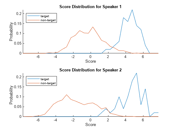
Analyze the equal error rate plots after applying adaptive s-norm1. The thresholds corresponding to the equal error rates for the two speakers are now closer together.
plotEER(targetScores,nontargetScores,Analyze="label")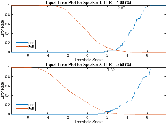
Analyze Score Normalization on Detection Error Tradeoff Set
Extract i-vectors from the DET set.
testIvecs = ivector(ivs,adsDET);
Place all of the enrolled i-vectors into a matrix.
enrolledIvecs = cat(2,ivs.EnrolledLabels.ivector{:});Calculate the normalization statistics for each enrolled and test i-vector. The supporting function, getNormFactors, performs the same operations as in Analyze Score Normalization on Two Speakers.
topK = 100;

normFactorsSe = getNormFactors(enrolledIvecs,imposterIvecs,TopK=topK);
normFactorsSt = getNormFactors(testIvecs,imposterIvecs,TopK=topK);
100;
normFactorsSe = getNormFactors(enrolledIvecs,imposterIvecs,TopK=topK);
normFactorsSt = getNormFactors(testIvecs,imposterIvecs,TopK=topK);Create a targets matrix indicating which i-vector pairs have corresponding labels.
targets = true(numel(adsDET.Labels),height(ivs.EnrolledLabels));
for ii = 1:height(ivs.EnrolledLabels)
    targets(:,ii) = ismember(adsDET.Labels,ivs.EnrolledLabels.Properties.RowNames(ii));
end
Score each enrollment i-vector against each test i-vector.
[targetScores,nontargetScores] = scoreTargets(enrolledIvecs,testIvecs,targets, ...
    NormFactorsSe=normFactorsSe,NormFactorsSt=normFactorsSt);
Plot the target and non-target score distributions for the group.
plotScoreDistributions(targetScores,nontargetScores,Analyze="group")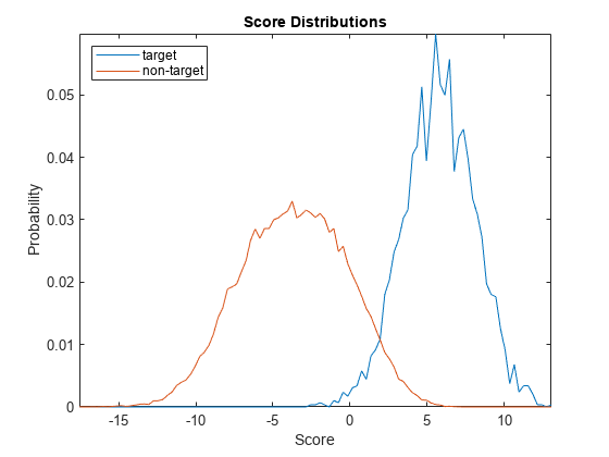
Plot the equal error rate of this new system. The equal error rate after applying adaptive s-norm1 is approximately 5 %. The equal error rate prior to adaptive s-norm1 is approximately 8 %.
plotEER(targetScores,nontargetScores,Analyze="group")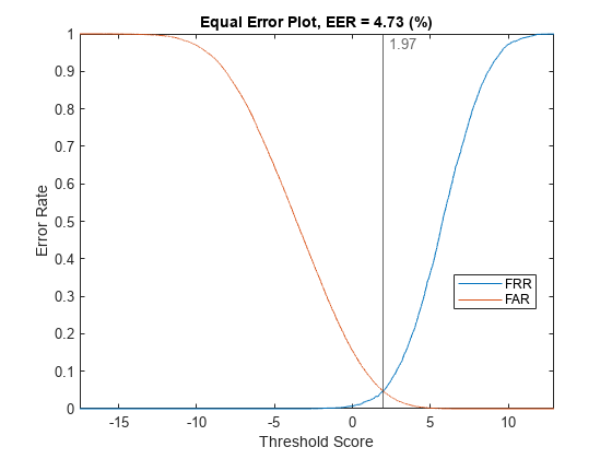
Supporting Functions
Load Dataset
function [adsEnroll,adsTest,adsDET,adsImposter] = loadDataset(targetSampleRate)
%LOADDATASET Load PTDB-TUG data set
% [adsEnroll,adsTest,adsDET,adsImposter] = loadDataset(targetSampleteRate)
% downloads the PTDB-TUG data set, resamples it to the specified target
% sample rate and save the results in your current folder. The function
% then creates and returns four audioDatastore objects. The enrollment set
% includes two utterances per speaker. The imposter set does not overlap
% with the other data sets.

% Copyright 2021-2022 The MathWorks, Inc.

arguments
    targetSampleRate (1,1) {mustBeNumeric,mustBePositive}
end

downloadFolder = matlab.internal.examples.downloadSupportFile("audio","ptdb-tug.zip");
dataFolder = tempdir;
unzip(downloadFolder,dataFolder)
dataset = fullfile(dataFolder,"ptdb-tug");

% Resample the dataset and save to current folder if it doesn't already
% exist.
if ~isfolder(fullfile(pwd,"MIC"))
    ads = audioDatastore([fullfile(dataset,"SPEECH DATA","FEMALE","MIC"),fullfile(dataset,"SPEECH DATA","MALE","MIC")], ...
        IncludeSubfolders=true, ...
        FileExtensions=".wav", ...
        LabelSource="foldernames");
    reduceDataset = false;
    if reduceDataset
        ads = splitEachLabel(ads,55);
    end
    adsTransform = transform(ads,@(x,y)fileResampler(x,y,targetSampleRate),IncludeInfo=true);

    writeall(adsTransform,pwd,OutputFormat="flac",UseParallel=~isempty(ver("parallel")))

end

% Create a datastore that points to the resampled dataset. Use the folder
% names as the labels.
ads = audioDatastore(fullfile(pwd,"MIC"),IncludeSubfolders=true,LabelSource="foldernames");

% Split the data set into enrollment, test, DET, and imposter sets.
imposterLabels = categorical(["M05","M10","F05","F10"]);
adsImposter = subset(ads,ismember(ads.Labels,imposterLabels));

adsDev = subset(ads,~ismember(ads.Labels,imposterLabels));
rng default
numToEnroll = 2;
[adsEnroll,adsDev] = splitEachLabel(adsDev,numToEnroll);

numToTest = 50;
[adsTest,adsDET] = splitEachLabel(adsDev,numToTest);
end
File Resampler
function [audioOut,adsInfo] = fileResampler(audioIn,adsInfo,targetSampleRate)
%FILERESAMPLER Resample audio files
% [audioOut,adsInfo] = fileResampler(audioIn,adsInfo,targetSampleRate)
% resamples the input audio to the target sample rate and updates the info
% passed through the datastore.

% Copyright 2021 The MathWorks, Inc.

arguments
    audioIn (:,1) {mustBeA(audioIn,["single","double"])}
    adsInfo (1,1) {mustBeA(adsInfo,"struct")}
    targetSampleRate (1,1) {mustBeNumeric,mustBePositive}
end

% Isolate the original sample rate
originalSampleRate = adsInfo.SampleRate;

% Resample if necessary
if originalSampleRate ~= targetSampleRate
    audioOut = resample(audioIn,targetSampleRate,originalSampleRate);
    amax = max(abs(audioOut));
    if max(amax>1)
        audioOut = audioOut./amax;
    end
end

% Update the info passed through the datastore
adsInfo.SampleRate = targetSampleRate;

end
Score Targets and Non-Targets
function [targetScores,nontargetScores] = scoreTargets(e,t,targetMap,nvargs)
%SCORETARGETS Score i-vector pairs
% [targetScores,nontargetScores] = scoreTargets(e,t,targetMap) exhaustively
% scores i-vectors in e against i-vectors in t. Specify e as an M-by-N
% matrix, where M corresponds to the i-vector dimension, and N corresponds
% to the number of i-vectors in e. Specify t as an M-by-P matrix, where P
% corresponds to the number of i-vectors in t. Specify targetMap as a
% P-by-N logical matrix that maps which i-vectors in e and t are target
% pairs (derived from the same speaker) and which i-vectors in e and t
% are non-target pairs (derived from different speakers). The
% outputs, targetScores and nontargetScores, are N-element cell arrays.
% Each cell contains a vector of scores between the i-vector in e and
% either all the targets or nontargets in t.
%
% [targetScores,nontargetScores] =
% scoreTargets(e,t,targetMap,NormFactorsSe=NFSe,NormFactorsSt=NFSt)
% normalizes the scores by the specified normalization statistics contained
% in structs NFSe and NFSt. If unspecified, no normalization is applied.

% Copyright 2021 The MathWorks, Inc.

arguments
    e (:,:) {mustBeA(e,["single","double"])}
    t (:,:) {mustBeA(t,["single","double"])}
    targetMap (:,:) {mustBeA(targetMap,"logical")}
    nvargs.NormFactorsSe = [];
    nvargs.NormFactorsSt = [];
end

% Score the i-vector pairs
scores = cosineSimilarityScore(e,t);

% Apply as-norm1 if normalization factors supplied
if ~isempty(nvargs.NormFactorsSe) && ~isempty(nvargs.NormFactorsSt)
    scores = 0.5*( (scores - nvargs.NormFactorsSe.mu)./nvargs.NormFactorsSe.std + (scores - nvargs.NormFactorsSt.mu')./nvargs.NormFactorsSt.std' );
end

% Separate the scores into targets and non-targets
targetScores = cell(size(targetMap,2),1);
nontargetScores = cell(size(targetMap,2),1);
for ii = 1:size(targetMap,2)
    targetScores{ii} = scores(targetMap(:,ii),ii);
    nontargetScores{ii} = scores(~targetMap(:,ii),ii);
end
end
Cosine Similarity Score (CSS)
function scores = cosineSimilarityScore(a,b)
%COSINESIMILARITYSCORE Cosine similarity score
% scores = cosineSimilarityScore(a,b) scores matrix of i-vectors, a,
% against matrix of i-vectors b. Specify a as an M-by-N matrix of
% i-vectors. Specify b as an M-by-P matrix of i-vectors. scores is returned
% as a P-by-N matrix, where columns corresponds the i-vectors in a
% and rows corresponds to the i-vectors in b and the elements of the array
% are the cosine similarity scores between them.

% Copyright 2021 The MathWorks, Inc.

arguments
    a (:,:) {mustBeA(a,["single","double"])}
    b (:,:) {mustBeA(b,["single","double"])}
end

scores = squeeze(sum(a.*reshape(b,size(b,1),1,[]),1)./(vecnorm(a).*reshape(vecnorm(b),1,1,[])));
scores = scores';
end
Plot Score Distributions
function plotScoreDistributions(targetScores,nontargetScores,nvargs)
%PLOTSCOREDISTRIBUTIONS Plot target and non-target score distributions
% plotScoreDistribution(targetScores,nontargetScores) plots empirical
% estimations of the distribution for target scores and nontarget scores.
% Specify targetScores and nontargetScores as cell arrays where each
% element contains a vector of speaker-specific scores.
%
% plotScoreDistrubtions(targetScores,nontargetScores,Analyze=ANALYZE)
% specifies the scope for analysis as either 'label' or 'group'. If ANALYZE
% is set to 'label', then a score distribution plot is created for each
% label. If ANALYZE is set to 'group', then a score distribution plot is
% created for the entire group by combining scores across speakers. If
% unspecified, ANALYZE defaults to 'group'.

% Copyright 2021 The MathWorks, Inc.

arguments
    targetScores (1,:) cell
    nontargetScores (1,:) cell
    nvargs.Analyze (1,:) char {mustBeMember(nvargs.Analyze,{'label','group'})} = 'group'
end

% Combine all scores to determine good bins for analyzing both the target
% and non-target scores together.
allScores = cat(1,targetScores{:},nontargetScores{:});
[~,edges] = histcounts(allScores);

% Determine the center of each bin for plotting purposes.
centers = movmedian(edges(:),2,Endpoints="discard");

if strcmpi(nvargs.Analyze,"group")
     % Plot the score distributions for the group.

    targetScoresBinCounts = histcounts(cat(1,targetScores{:}),edges);
    targetScoresBinProb = targetScoresBinCounts(:)./sum(targetScoresBinCounts);
    nontargetScoresBinCounts = histcounts(cat(1,nontargetScores{:}),edges);
    nontargetScoresBinProb = nontargetScoresBinCounts(:)./sum(nontargetScoresBinCounts);

    figure
    plot(centers,[targetScoresBinProb,nontargetScoresBinProb])
    title("Score Distributions")
    xlabel("Score")
    ylabel("Probability")
    legend(["target","non-target"],Location="northwest")
    axis tight

else

    % Create a tiled layout and plot the score distributions for each speaker.
    N = numel(targetScores);
    tiledlayout(N,1)
    for ii = 1:N
        targetScoresBinCounts = histcounts(targetScores{ii},edges);
        targetScoresBinProb = targetScoresBinCounts(:)./sum(targetScoresBinCounts);
        nontargetScoresBinCounts = histcounts(nontargetScores{ii},edges);
        nontargetScoresBinProb = nontargetScoresBinCounts(:)./sum(nontargetScoresBinCounts);

        nexttile
        hold on
        plot(centers,[targetScoresBinProb,nontargetScoresBinProb])
        title("Score Distribution for Speaker " + string(ii))
        xlabel("Score")
        ylabel("Probability")
        legend(["target","non-target"],Location="northwest")
        axis tight
    end
end
end
Plot Equal Error Rate (EER)
function plotEER(targetScores,nontargetScores,nvargs)
%PLOTEER Plot equal error rate (EER)
% plotEER(targetScores,nontargetScores) creates an equal error rate plot
% using the target scores and the non-target scores. Specify targetScores
% and nontargetScores as cell arrays where each element contains a vector
% of speaker-specific scores.
%
% plotEER(targetScores,nontargetScores,Analyze=ANALYZE) specifies the
% scope for analysis as either 'label' or 'group'. If ANALYZE is set to
% 'label', then an equal error rate plot is created for each label. If
% ANALYZE is set to 'group', then an equal error rate plot is created for
% the entire group by combining scores across speakers. If unspecified,
% ANALYZE defaults to 'group'.

% Copyright 2021 The MathWorks, Inc.

arguments
    targetScores (1,:) cell
    nontargetScores (1,:) cell
    nvargs.Analyze (1,:) char {mustBeMember(nvargs.Analyze,{'label','group'})} = 'group'
end

% Combine all scores to determine good bins for analyzing both the target
% and non-target scores together.
allScores = cat(1,targetScores{:},nontargetScores{:});
[~,edges] = histcounts(allScores,BinWidth=0.002);

% Determine the center of each bin for plotting purposes.
centers = movmedian(edges(:),2,Endpoints="discard");

if strcmpi(nvargs.Analyze,"group")
    % Plot the equal error rate for the group.

    targetScoresBinCounts = histcounts(cat(1,targetScores{:}),edges);
    targetScoresBinProb = targetScoresBinCounts(:)./sum(targetScoresBinCounts);
    nontargetScoresBinCounts = histcounts(cat(1,nontargetScores{:}),edges);
    nontargetScoresBinProb = nontargetScoresBinCounts(:)./sum(nontargetScoresBinCounts);

    targetScoresCDF = cumsum(targetScoresBinProb);
    nontargetScoresCDF = cumsum(nontargetScoresBinProb,"reverse");
    [~,idx] = min(abs(targetScoresCDF(:) - nontargetScoresCDF));

    figure
    plot(centers,[targetScoresCDF,nontargetScoresCDF])
    xline(centers(idx),"-",num2str(centers(idx),3),LabelOrientation="horizontal")
    legend(["FRR","FAR"],Location="best")
    xlabel("Threshold Score")
    ylabel("Error Rate")
    title(sprintf("Equal Error Plot, EER = %0.2f (%%)",100*mean([targetScoresCDF(idx);nontargetScoresCDF(idx)])))
    axis tight

else

    % Create a tiled layout and plot the equal error rate for each speaker.
    N = numel(targetScores);
    f = figure;
    tiledlayout(f,N,1,Padding="tight",TileSpacing="tight")
    for ii = 1:N
        targetScoresBinCounts = histcounts(targetScores{ii},edges);
        targetScoresBinProb = targetScoresBinCounts(:)./sum(targetScoresBinCounts);
        nontargetScoresBinCounts = histcounts(nontargetScores{ii},edges);
        nontargetScoresBinProb = nontargetScoresBinCounts(:)./sum(nontargetScoresBinCounts);

        targetScoresCDF = cumsum(targetScoresBinProb);
        nontargetScoresCDF = cumsum(nontargetScoresBinProb,"reverse");
        [~,idx] = min(abs(targetScoresCDF(:) - nontargetScoresCDF));

        nexttile
        plot(centers,[targetScoresCDF,nontargetScoresCDF])
        xline(centers(idx),"-",num2str(centers(idx),3),LabelOrientation="horizontal")
        legend(["FRR","FAR"],Location="southwest")
        xlabel("Threshold Score")
        ylabel("Error Rate")
        title(sprintf("Equal Error Plot for Speaker " + string(ii) + ", EER = %0.2f (%%)", ...
            100*mean([targetScoresCDF(idx);nontargetScoresCDF(idx)])))
        axis tight
    end
end
end
Get Norm Factors
function normFactors = getNormFactors(w,imposterCohort,nvargs)
%GETNORMFACTORS Get norm factors
% normFactors = getNormFactors(w,imposterCohort) returns the mean and
% standard deviation of the scores between the i-vectors in w and the i-vectors
% in the imposter cohort. Specify w as a matrix of i-vectors. Specify
% imposterCohort as a matrix of i-vectors. Each column corresponds to an
% i-vector the same length as w.
%
% normFactors = getNormFactors(w,imposterCohort,TopK=TOPK) calculates the
% normalization statistics using only the top K highest scores. If
% unspecified, all scores are used.

% Copyright 2021 The MathWorks, Inc.

arguments
    w (:,:) {mustBeA(w,["single","double"])}
    imposterCohort (:,:) {mustBeA(imposterCohort,["single","double"])}
    nvargs.TopK (1,1) {mustBePositive} = inf
end
topK = min(ceil(nvargs.TopK),size(imposterCohort,2));

% Score the template i-vector against the imposter cohort.
imposterScores = cosineSimilarityScore(w,imposterCohort);

% Isolate the top K scores.
imposterScores = sort(imposterScores,"descend");
imposterScores = imposterScores(1:topK,:);

% Calculate the score normalization statistics
MU = mean(imposterScores,1);
STD = std(imposterScores,[],1);

% Return normalization statistics as a struct
normFactors = struct(mu=MU,std=STD);
end
References
[1] Matejka, Pavel, Ondrej Novotny, Oldrich Plchot, Lukas Burget, Mireia Diez Sanchez, and Jan Cernocky. "Analysis of Score Normalization in Multilingual Speaker Recognition." Interspeech 2017, 2017. https://doi.org/10.21437/interspeech.2017-803.
[2] van Leeuwen, David A., and Niko Brummer. "An Introduction to Application-Independent Evaluation of Speaker Recognition Systems." Lecture Notes in Computer Science, 2007, 330–53. https://doi.org/10.1007/978-3-540-74200-5_19.
[3] G. Pirker, M. Wohlmayr, S. Petrik, and F. Pernkopf, "A Pitch Tracking Corpus with Evaluation on Multipitch Tracking Scenario", Interspeech, pp. 1509-1512, 2011.