getrom

Obtain reduced-order models when using frequency-response fitting method

Since R2025a

Syntax

rsys = getrom(R)

rsys = getrom(R,Name=Value)

Description

rsys = getrom(R) returns a stable explicit state-space model rsys of the rational fit R.Fit.

rsys = getrom(R,Name=Value) returns a reduced-order model rsys based on the options specified by one or more name-value arguments.

Examples

Reduce Sparse Model Order Using Frequency Response Fitting Method

This example shows how to reduce model order of a sparss model using the frequency response fitting method. The sparse state-space model used in this example is obtained from linearizing a thermal model of heat distribution in a circular cylindrical rod.

Load the model data.

load cylindricalRod.mat
sys = sparss(A,B,C,D,E);
size(sys)

Sparse state-space model with 3 outputs, 1 inputs, and 7522 states.

The thermal model contains 7522 states.

To reduce the model order, first create a frequency response fitting specification object for sys.

R = reducespec(sys,'frfit');

To customize the specification object, you can specify additional options such as a frequency grid and the feedthrough values. Since the feedthrough values for the original model is zero, you can set it to zero in the options.

w = logspace(-7,-3,20);
R.Options.Frequency = w;
R.Options.Feedthrough = zeros(3,1);
R.Options.RelTol = 1e-3;
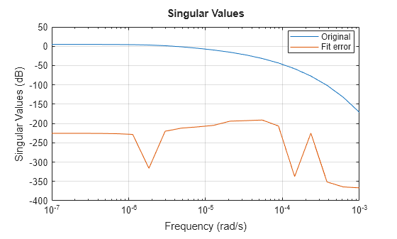
R.Options.Display = 'off';

Run the model reduction algorithm and visualize the frequency response of the original model and the fit error.

R = process(R);
view(R)

Obtain the reduced model from the rational fit. You can specify additional arguments of getrom such that the software returns a model in descriptor form and does not enforce any stability on the fitted model.

rsys = getrom(R,Explicit=false,Stable=false);
order(rsys)

ans = 
11

Compare the relative error between two models.

sigmaplot(sys,sys-rsys,"r--",w)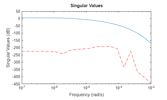

The reduced model provides a good approximation of the original sparse model.

Fit Low-Order Model to Frequency Response of Tuning Fork Sparse Model

This example shows how to fit a low-order model using the frequency response fitting method. In this example, you obtain a reduced-order model of a tuning fork model. The model is a sparse second-order (mechss) model with two outputs, one input, and 3024 degrees of freedom.

Load the model.

load tuningForkData.mat
sys = mechss(M,[],K,B,F);
w = logspace(2,6,250);
size(sys)

Sparse second-order model with 2 outputs, 1 inputs, and 3024 degrees of freedom.

Create a model order reduction object for frequency response fitting using reducespec. Specify a frequency grid and the feedthrough value for interpolation.

R = reducespec(sys,'frfit');
R.Options.Frequency = w;
R.Options.Feedthrough = [0;0];
R.Options.Display = "off";
R = process(R);

rsys1 = getrom(R,Explicit=false,Stable=true,Minimal=true);
o1 = order(rsys1)

o1 = 
90

sigmaplot(sys,rsys1,"--",w)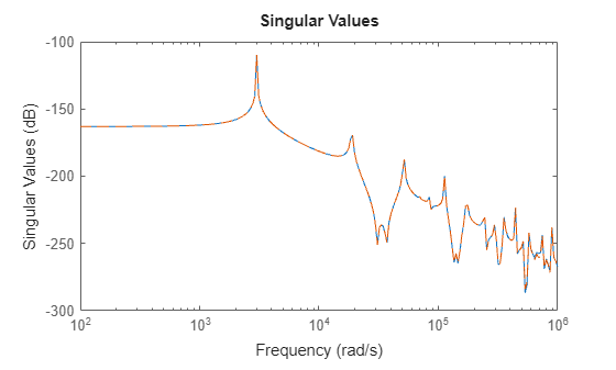

This returns a model with an order which is still quite high. You can further reduce the model order by focusing on just the lower frequencies. Increasing AbsTol allows for a larger error at higher frequencies where the gain is low but the mode density increases.

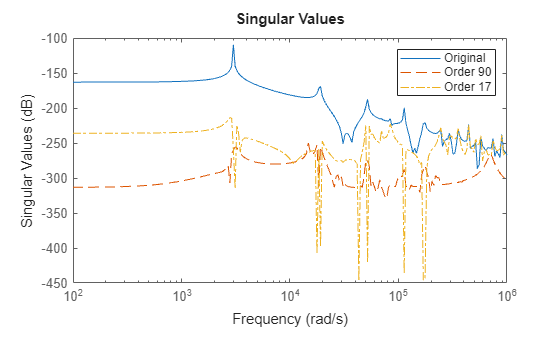
R.Options.AbsTol = 1e-11;
R.Options.RelTol = 1e-3;
rsys2 = getrom(R,Explicit=false,Stable=true,Minimal=true);
o2 = order(rsys2)

o2 = 
17

The algorithm now produces a reduced model with much lower order. Compare the relative error between the original and reduced models.

sigmaplot(sys,sys-rsys1,"--",sys-rsys2,"-.",w)
legend("Original",sprintf("Order %d",o1),...
    sprintf("Order %d",o2));

Reduce MIMO Model Using Frequency Response Fitting

This example shows how to reduce a model order of a multi-input multi-output (MIMO) model using the frequency response fitting method. Typically, when you reduce MIMO models using this method, the default reduced model may not have a minimal order. This example shows how to ensure the fit is minimal.

For this example, generate a random state-space model with 50 states, two outputs, and three inputs.

rng(0);
sys = rss(50,2,3);

When using the frequency response fitting method, the software requires you to specify a grid of frequencies for evaluating the frequency response. To select a suitable grid, analyze the frequency response of the model.

sigmaplot(sys)

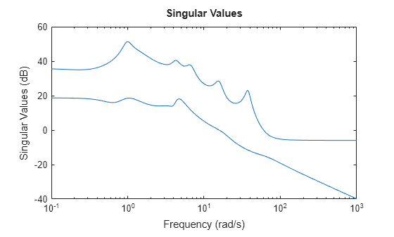
For this model, you can specify frequencies between 0.1 rad/s and 1000 rad/s.

w = logspace(-1,3,100);

Create a model reduction object.

R = reducespec(sys,"frfit");

Specify the desired frequency grid and run the model reduction algorithm.

R.Options.Frequency = w;
R = process(R);

Obtain the reduced model from the rational fit.

rsys = getrom(R);
order(rsys)

ans = 
30

This produces a 30th order model. By default, getrom returns a stable and explicit realization of the reduced model. However, when you use this method with MIMO models, the software may produce a nonminimal order fit. To ensure a minimal order fit, you can set the Minimal argument of getrom to true. This performs an additional balanced truncation on the initially reduced model. The software further reduces this model as long as it maintains the desired fit accuracy.

Obtain the model.

rsys2 = getrom(R,Minimal=true);
order(rsys2)

ans = 
26

Now getrom produces a model with order 26. Compare the relative error between the original and reduced models.

sigmaplot(sys,sys-rsys,":",sys-rsys2,"--")
legend("sys","sys-rsys","sys-rsys2")

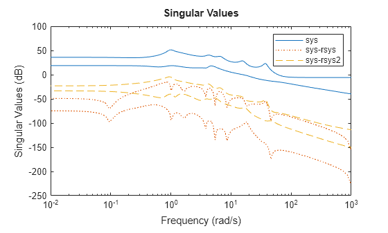
The fitted models provide an accurate match for the original model.

Enforcing Stability in Fitted Reduced Models

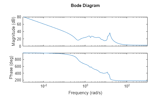
This example shows how to enforce stability in reduced models obtained using frequency response fitting method and the effects of refining the frequency grid to avoid unstable modes.

Generate a random state-space model.

rng(1) 
sys = rss(50);  
bodeplot(sys)

First, reduce the model using a frequency grid of 30 points between 0.01 rad/s and 100 rad/s.

w = logspace(-2,2,30);
R = reducespec(sys,'frfit');
R.Options.Frequency = w;

When you use getrom with the Stable argument set to false, the software runs the standard AAA algorithm which does not enforce stability of the fitted model.

rsys1 = getrom(R,Stable=false);

The low relative error shows that the reduced model is a good fit on the specified grid.

sigma(sys,sys-rsys1,w)
legend("sys","sys-rsys1",Location="best")

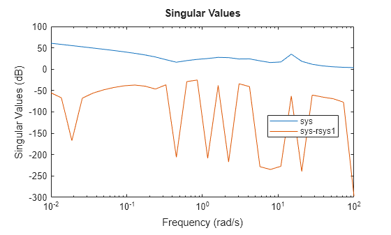
However, outside the grid points, the reduced model does not provide a good fit.

bode(sys,rsys1)
legend

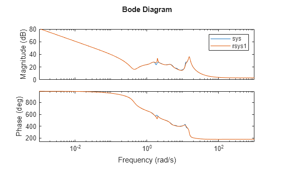
Additionally, this fit is also unstable.

max(real(pole(rsys1)))

ans = 
0.0335

However, when Stable is set to true, the software enforces stability after the AAA algorithm has run.

rsys2 = getrom(R,Stable=true);
max(real(pole(rsys2)))

ans = 
-2.9364e-08

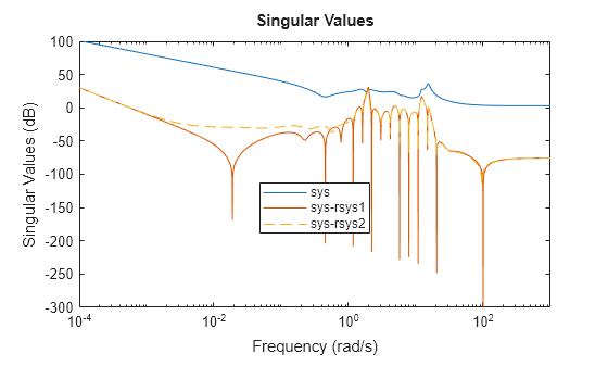
In this case, the stabilization works well with only a minor degradation in fit quality. This is not always the case however, post-AAA stabilization may introduce significant errors past the frequency of the first stabilized mode.

sigma(sys,sys-rsys1,sys-rsys2,"--")
legend("sys","sys-rsys1","sys-rsys2",Location="best")

In principle, stability is encoded in the frequency response. In general, unstable poles creep in where the frequency grid is too sparse to accurately capture the system dynamics. Refining the grid is often an effective, error-free way to restore stability

w = logspace(-2,2,60);
R = reducespec(sys,'frfit');
R.Options.Frequency = w;
rsys3 = getrom(R,Stable=false);
max(real(pole(rsys3)))

ans = 
3.3737e-08

This last fit rsys3 is stable and more accurate than the stabilized fit rsys2.

sigma(sys,sys-rsys2,sys-rsys3,"--")
legend("sys","sys-rsys2","sys-rsys3",Location="best")

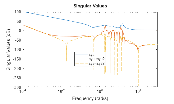
There is a small increase in order for the refined grid as there is more data to fit.

[order(rsys2) order(rsys3)]

ans = 1×2

    17    19

Therefore, when a stable model is required and getrom returns an unstable fit, you can either enforce stability with Stable=true, or refine the grid.

Input Arguments

R — Model order reduction specification object

FrequencyResponseFitting object

Model order reduction specification object created using reducespec, specified as a FrequencyResponseFitting object.

Name-Value Arguments

Specify optional pairs of arguments as Name1=Value1,...,NameN=ValueN, where Name is the argument name and Value is the corresponding value. Name-value arguments must appear after other arguments, but the order of the pairs does not matter.

Example: rsys = getrom(R,Explicit=false)

Explicit — Return explicit model

true (default) | false

Option to return the state-space realization in explicit form, specified as true or false. When you set this option to true, the function returns the reduced model in an explicit state-space realization, otherwise it returns the model in a descriptor state-space realization.

Stable — Return stable state-space model

true (default) | false

Option to return a stable state-space model, specified as true or false. Stability is encoded in the frequency response, but coarse frequency sampling may lose this information and the software may produce unstable fits. When you set this option to true, the software enforces stability on the model, but this can degrade the fit quality. You can rectify this by increasing the frequency grid density near the underdamped poles (resonances in the frequency response). However, the more frequency points you have, the longer it takes to evaluate the frequency response.

Minimal — Minimize fit order while maintaining desired accuracy

false (default) | true

Minimize fit order while maintaining desired accuracy, specified as true or false. When you set this option to true, the function applies balanced truncation on the initial fit to eliminate redundant dynamics. By default, the function is not guaranteed produce a minimal order fit especially for multi-input multi-output models. Therefore, enable this option to minimize the fit order.

Output Arguments

rsys — Reduced-order model

state-space model

Reduced-order model, returned as a state-space model.

Version History

Introduced in R2025a