Proper Orthogonal Decomposition Using Model Reducer

Since R2025a

This example shows how to reduce model order using the Proper Orthogonal Decomposition (POD) method in the Model Reducer app. POD is a simulation-based technique to extract dominant state directions and perform an approximate balanced truncation. This method takes snapshots of the state vector during simulation and uses principal component analysis (PCA) to obtain the principal state directions.

For this example, consider a a three-story building model described in the Active Vibration Control in Three-Story Building example. The model has 20 outputs, 2 inputs, and 30 states. Since POD is a simulation-based technique, reducing models with a large number of inputs and output can be inefficient. This example shows how to configure options when you want you reduce order of such models.

Load the model data.

load threeStoryBuilding.mat
size(PF)

State-space model with 20 outputs, 2 inputs, and 30 states.

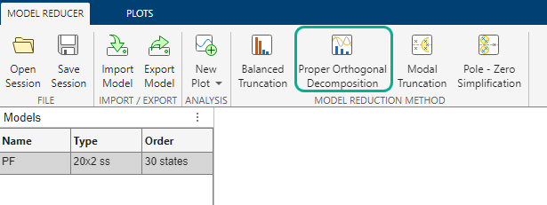
Open the app, and import the model to reduce.

modelReducer(PF)

To launch POD reduction, on the Model Reducer tab, click Proper Orthogonal Decomposition.

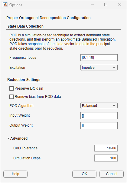
Before proceeding with POD reduction, you must first specify options. The software allows you to specify options such as frequency focus, excitation signal for simulation, and POD algorithm. For more information about available options, see Specify Options for Proper Orthogonal Decomposition in Model Reducer.

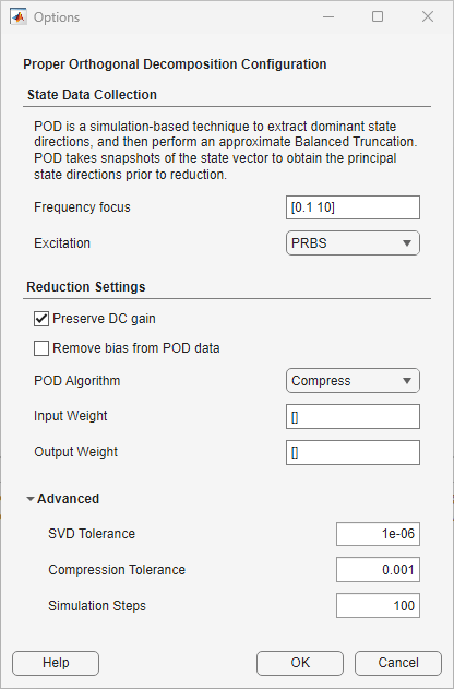
Since this is a model with many outputs and just two inputs, one way to avoid running several simulations is to use the Compress algorithm. The Compress algorithm is an acceleration of Balanced algorithm for tall or wide models (few inputs, many outputs or few outputs, many inputs). The algorithm runs the cheapest simulation (input-to-state if few inputs), uses the resulting POD of state-snapshots to compress the output and find the dominant output directions, and then performs the adjoint simulation with this reduced output.

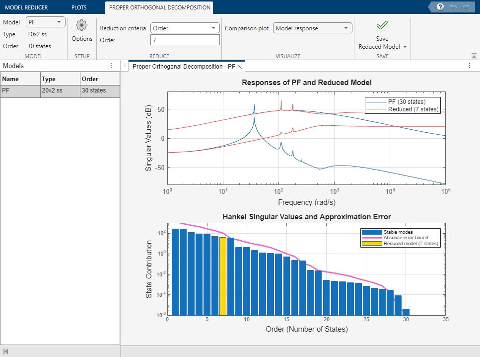
Set the options as shown in the following figure and click OK.

By default, the Model Reducer app selects order 7. The resulting reduced model does not provide a good approximation of the original model.

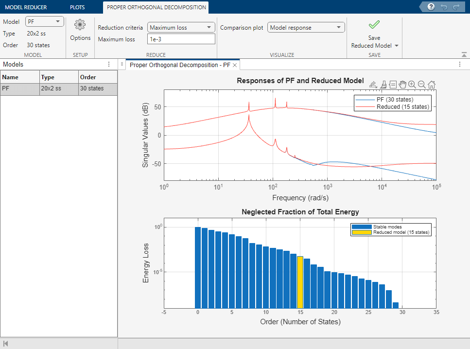
To get a better approximation, set Reduction criteria to Maximum loss with a value of 1e-3. Doing so allows you to obtain a reduced model that neglects 0.1% of the total energy. This results in a 15th-order model and a much better approximation.

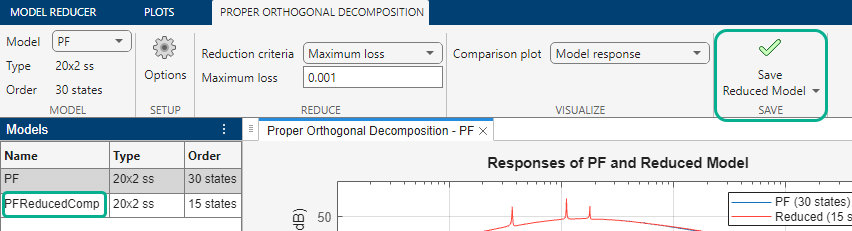
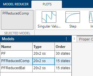
To save the reduced model in the app workspace, click Save Reduced Model. Click the saved model and rename it to PFReducedComp.

Alternatively, if you know the critical or dominant inputs and outputs through physical insights, you can use input and and output weights to reduce I/O dimension. For this model, select the outputs 13, 14, 15 which correspond to the inter-story drift in the building, and emphasize input 1 which is the ground acceleration during an earthquake. First create the weights, and then click Options on the Proper Orthogonal Decomposition tab to open the options dialog.

Wy = zeros(3,20);
Wy(:,13:15) = eye(3);
Wu = [1e3;1];

Specify the options as shown in the following figure. When using the Balanced algorithm, the software considers both the input-to-state and state-to-output maps (through the adjoint simulation) to approximate the reachability and observability Gramians. Therefore, reducing I/O dimensions using weights to account only for dominant inputs and outputs may increase the efficiency of the algorithm.

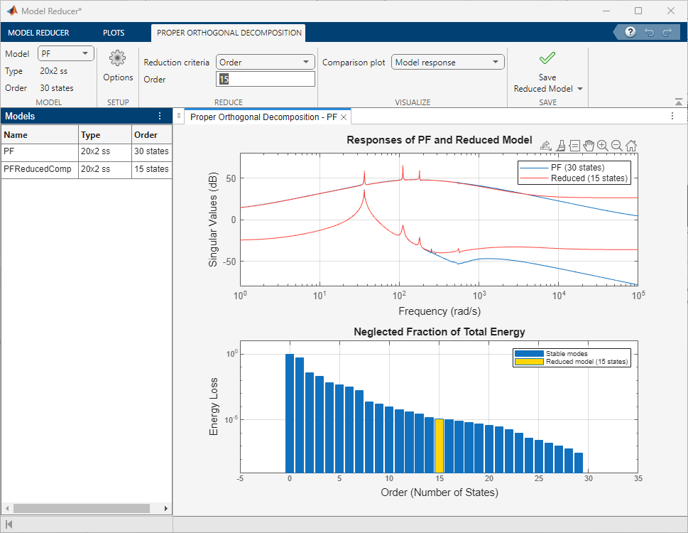
Click OK and specify a model order of 15 to obtain the model of same order as the model obtained with the Compress algorithm in the previous section.

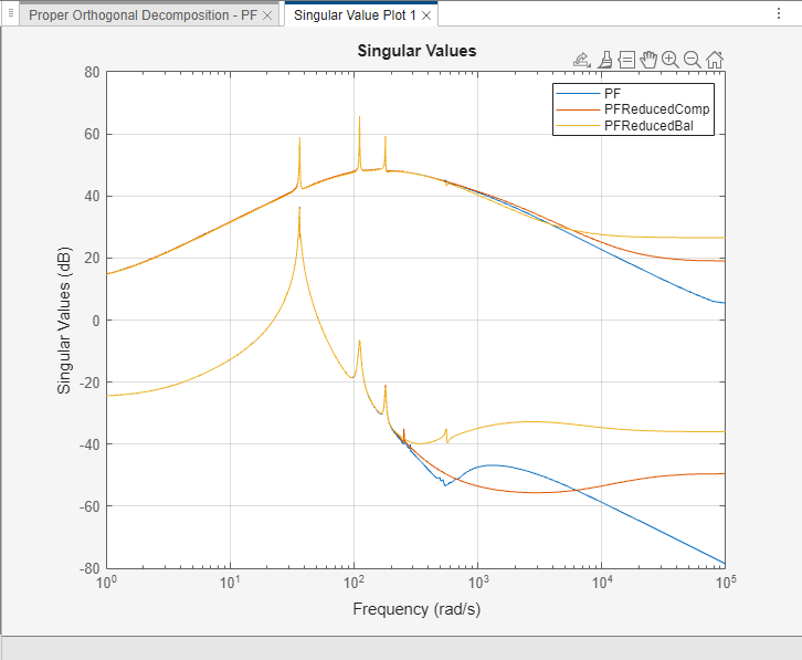
Save the model and rename it to PFReducedBal. You can compare the original model with the two reduced models. Click the Plots tab and select the Singular Value plot.

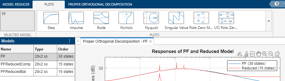
In the Models workspace, click PFReducedComp and select Singular Value Plot 1 to add the model to the existing plot.

Similarly, to compare all three models, add the PFReducedBal reduced model to the same plot. You can see that both reduction methods provide a good approximation of the original model and confirms that the emphasized input-output channels in the Balanced algorithm contribute to the majority of system dynamics.