Tune Compression Parameters for Sequence Classification Network for Road Damage Detection

Since R2025a

This example uses:

This example shows how to tune the relative amounts of pruning and projection to optimize accuracy when compressing a network to meet a fixed memory requirement using Experiment Manager.

This example is step three in a series of examples that shows how to train and compress a neural network. You can run each step independently or work through the steps in order.

In the previous example, you compress a neural network using a combination of pruning, projection, and quantization. You can achieve the same compressed network size by using different ratios of pruning and projection. For example, you can only prune and not project, or remove equal numbers of parameters using either method. In the previous example, you use an arbitrary split between pruning and projection.

In this example, you use Experiment Manager to determine what combination of pruning and projection results in the best accuracy while meeting a fixed memory requirement.

Create Experiment Manager Project

First, open Experiment Manager by running experimentManager in the MATLAB® Command Window or by opening the Experiment Manager App from the Apps tab.

>> experimentManager

In Experiment Manager, select New and then Project. After a new window opens, select Blank Project and then General Purpose. Click Add. Enter a name for the experiment.

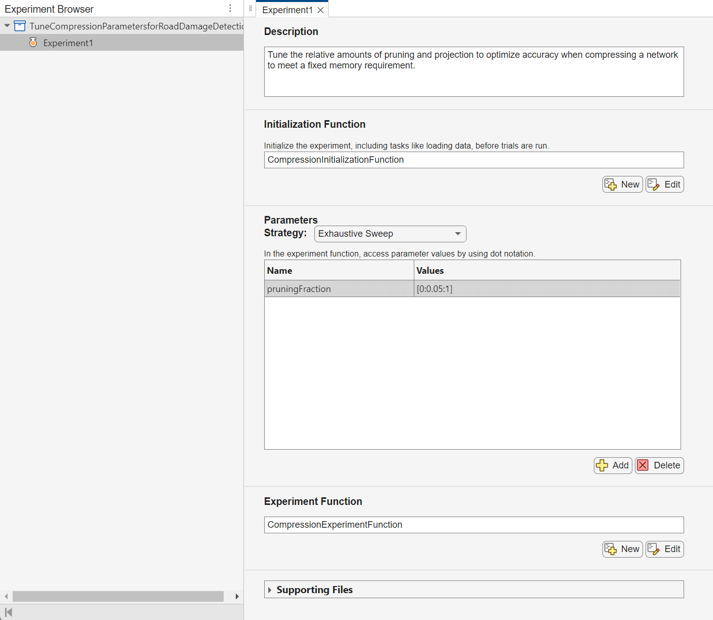
Next, to configure the experiment, perform these steps.

Optionally, add a description.
Add the Initialization Function — In the Initialization Function section, select New. Name the function CompressionInitializationFunction. Delete the contents. Then, copy the contents of the CompressionInitializationFunction function, defined at the bottom of this example, and paste them into the newly created CompressionInitializationFunction. Save the function.
Add the pruning fraction parameter — In the Parameters section, add a new parameter. Name it pruningFraction with values [0:0.05:1]. To assess each value of the pruningFraction parameter, keep the exhaustive sweep strategy. This parameter determines what fraction of learnable parameters are removed using pruning. For more information, see Compress Sequence Classification Network for Road Damage Detection.
Add the Experiment Function — In the Experiment Function section, select New. Name the function CompressionExperimentFunction. Delete the contents. Then, copy the contents of the CompressionExperimentFunction function, defined at the bottom of this example, and paste them into the newly created CompressionExperimentFunction. Save the function.
Add the supporting files — Copy the files countTotalParameters.m, loadAndPreprocessDataForRoadDamageDetectionExample.m, and RoadDamageAnalysisNetwork.mat, attached to this example as supporting files, to the project directory created by Experiment Manager. Experiment Manager automatically detects the supporting files in the project directory.

Run Experiment

To run the experiment, click Run.

If you have a GPU available, then you can run the experiments in parallel by first setting the mode to Simultaneous and then clicking Run.

Export Trial with Best Accuracy

Once the experiment has run, choose the trial that results in the best accuracy while still meeting the memory requirement. To sort the trials by accuracy, hover over the column header accuracyNetQuantized. Click the downward arrow and select Sort in Descending Order.

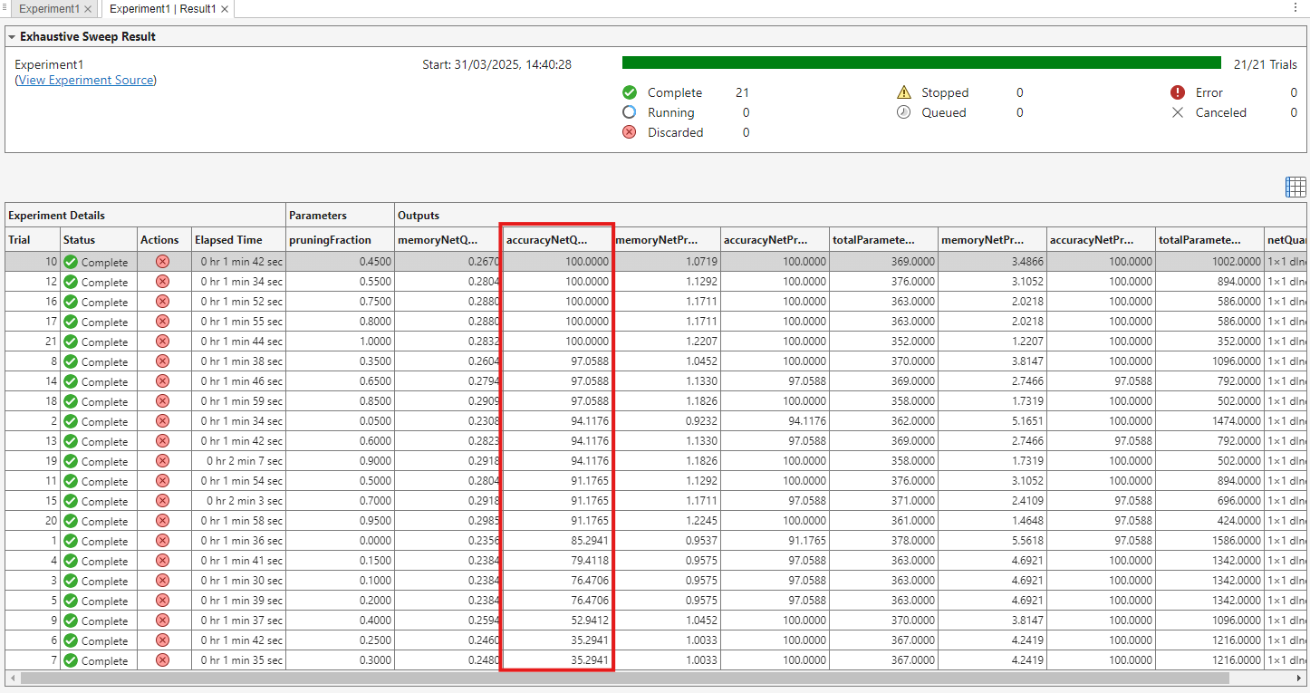
To enable you to run this example quickly, the network and data set are small. Due to the small network and data set, the results of the experiment can vary.

In this run of the experiment, trials 10, 12, 16, 17 and 21 are tied for the best accuracy after quantization. Trial 10 with a pruning fraction of 0.45 results in the smallest network after quantization. This value corresponds to 45% pruning and 55% projection. The data from this trial, including the resulting network, is attached to this example as a supporting file, trialBestAccuracy.mat.

The estimateLayerMemory function, defined at the bottom of this example, uses the estimateNetworkMetrics function to measure the memory of each supported layer. The batch normalization layers in the network are not supported, so the resulting number is less than the total network memory. For a list of supported layers, see estimateNetworkMetrics.

To export the trial with the best accuracy to the workspace, first select the trial in the results table. Then, select Export and click Export Selected Trial. Name the variable trialBestAccuracy. Save the variable to a MAT (*.mat) file.

>> save("trialBestAccuracy","trialBestAccuracy")

Test Compressed Network

Load the uncompressed network and data. Load the compressed network, memory, and accuracy information of the trial with the best accuracy.

load("RoadDamageAnalysisNetwork.mat")
loadAndPreprocessDataForRoadDamageDetectionExample
load("trialBestAccuracy.mat")

Make predictions using the minibatchpredict function and convert the scores to labels using the onehotdecode function. By default, the minibatchpredict function uses a GPU if one is available.

YTest = minibatchpredict(trialBestAccuracy.Outputs.netQuantized{1},XTest);
YTestLabels = onehotdecode(YTest,labels,1);
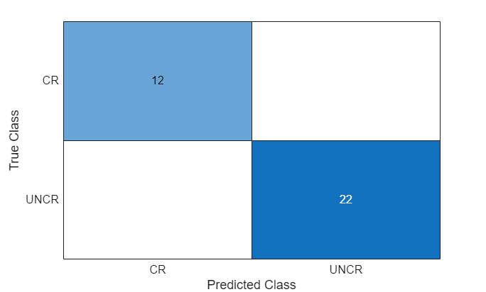
TTestLabels = onehotdecode(TTest,labels,1);

Display the classification results in a confusion chart.

figure
confusionchart(TTestLabels,YTestLabels)

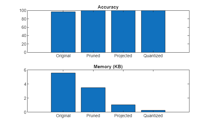
Compare accuracy and memory after each compression step.

memoryNetTrained = estimateLayerMemory(netTrained);
accuracyNetTrained = testnet(netTrained,XTest,TTest,"accuracy");
memory = [memoryNetTrained,trialBestAccuracy.Outputs.memoryNetPruned,trialBestAccuracy.Outputs.memoryNetProjected,trialBestAccuracy.Outputs.memoryNetQuantized];
accuracy = [accuracyNetTrained,trialBestAccuracy.Outputs.accuracyNetPruned,trialBestAccuracy.Outputs.accuracyNetProjected,trialBestAccuracy.Outputs.accuracyNetQuantized];

Plot accuracy and memory after each compression step.

figure
tiledlayout("vertical")
t1 = nexttile;
bar(t1,accuracy)
title(t1,"Accuracy")
xticklabels(["Original" "Pruned" "Projected" "Quantized"])

t2 = nexttile;
bar(t2,memory)
title(t2,"Memory (KB)")
xticklabels(["Original" "Pruned" "Projected" "Quantized"])

In the next step in this workflow, you automatically generate a Simulink® model from the quantized network in this example.

Next step: Generate Simulink Model from Sequence Classification Network for Road Damage Detection. You can also open the next example using the openExample function.

>> openExample('deeplearning_shared/GenerateSimulinkModelFromRoadDamageAnalysisNetworkExample')

Helper Function

function layerMemoryInKB = estimateLayerMemory(net)
    info = estimateNetworkMetrics(net);
    layerMemoryInMB = sum(info.("ParameterMemory (MB)"));
    layerMemoryInKB = layerMemoryInMB * 1000;
end

Initialization Function

The initialization function runs once at the start of the experiment. The function performs these steps as described in the Compress Sequence Classification Network for Road Damage Detection example.

Load the trained network and data.
Set the compression goal.
Calculate the total number of parameters to remove using pruning and projection.

The function returns these variables in a single output structure array.

The initialization function in this example was created from the Compress Sequence Classification Network for Road Damage Detection example using these steps.

Create a function called CompressionInitializationFunction with no input arguments and a single output argument output.
Copy the code from the example before the definition of the pruningFraction parameter into the body of the function.
Suppress any outputs. Do not display plots during training.
Add these parameters to the output structure output: XTrain, TTrain, XValidation, TValidation, XTest, TTest, netTrained, options, lossFcn, totalParametersReductionGoal, and totalParametersGoal.

function output = CompressionInitializationFunction()

load("RoadDamageAnalysisNetwork.mat")
loadAndPreprocessDataForRoadDamageDetectionExample

output.XTrain = XTrain;
output.TTrain = TTrain;
output.XValidation = XValidation;
output.TValidation = TValidation;
output.XTest = XTest;
output.TTest = TTest;
output.netTrained = netTrained;
output.options = options;
output.lossFcn = lossFcn;

output.options.Plots = "none";

memoryUncompressed = 6.2;
memoryGoal = 1.5;
output.totalParametersReductionGoal = (memoryUncompressed - memoryGoal) / memoryUncompressed;
totalParametersNetTrained = countTotalParameters(output.netTrained);
output.totalParametersGoal = floor(totalParametersNetTrained * (1 - output.totalParametersReductionGoal));

end

Experiment Function

The experiment function runs once per trial. The function performs these steps as described in the Compress Sequence Classification Network for Road Damage Detection example.

Prune and retrain the network.
Project and retrain the network.
Quantize the network.

For an example showing how to create an experiment function from a MATLAB script, see Convert MATLAB Code into Experiment.

The experiment function in this example was created from Compress Sequence Classification Network for Road Damage Detection example using these steps.

Create a function called CompressionExperimentFunction with a single input argument params and these output arguments: memoryNetQuantized, accuracyNetQuantized, memoryNetProjected, accuracyNetProjected, totalParametersNetProjected, memoryNetPruned, accuracyNetPruned, totalParametersNetPruned, and netQuantized. If your network is large, then returning the quantized network in the experiment function can take up a lot of memory. Instead, you can compress the network after the experiment using the hyperparameters that resulted in the best accuracy during the experiment.
Copy the contents of the example script after the definition of the pruningFraction parameter and before the section Test Results into the body of the function.
Disable the training plots and suppress any outputs.
Rename pruningFraction to params.pruningFraction. This expression uses dot notation to access the parameter values that you specify in the Parameters section in Experiment Manager.
Rename the parameters created in the initialization function. For example, replace netTrained with params.InitializationFunctionOutput.netTrained. This expression uses dot notation to access the output values of the initialization function.

function [memoryNetQuantized,accuracyNetQuantized, ...
    memoryNetProjected,accuracyNetProjected,totalParametersNetProjected, ...
    memoryNetPruned,accuracyNetPruned,totalParametersNetPruned, ...
    netQuantized] = CompressionExperimentFunction(params)

% Prune
totalParametersNetTrained = countTotalParameters(params.InitializationFunctionOutput.netTrained);
pruningTotalParametersGoal = floor(totalParametersNetTrained * (1 - params.InitializationFunctionOutput.totalParametersReductionGoal * params.pruningFraction));
numRetrainingEpochs = 15;
initialLearnRate = 0.01;
maxFiltersToPrunePerIteration = 2;
doPrune = true;
netPrunable = taylorPrunableNetwork(params.InitializationFunctionOutput.netTrained);
totalParametersNetPruned = totalParametersNetTrained;
if canUseGPU
    XTrain = gpuArray(params.InitializationFunctionOutput.XTrain);
    TTrain = gpuArray(params.InitializationFunctionOutput.TTrain);
end
while (totalParametersNetPruned > pruningTotalParametersGoal) && doPrune
    averageGrad = [];
    averageSqGrad = [];
    fineTuningIteration = 0;  
    for jj = 1:numRetrainingEpochs
        fineTuningIteration = fineTuningIteration+1;        
        [~,state,gradients,pruningActivations,pruningGradients] = dlfeval(@modelLoss,netPrunable,params.InitializationFunctionOutput.XTrain,params.InitializationFunctionOutput.TTrain,params.InitializationFunctionOutput.lossFcn);        
        netPrunable.State = state;
        [netPrunable,averageGrad,averageSqGrad] = adamupdate(netPrunable, gradients, ...
            averageGrad,averageSqGrad, fineTuningIteration, initialLearnRate);
        if jj==numRetrainingEpochs
            netPrunable = updateScore(netPrunable,pruningActivations,pruningGradients);
        end
    end
    netPrunable = updatePrunables(netPrunable,MaxToPrune=maxFiltersToPrunePerIteration);
    updatedTotalParameters = countTotalParameters(netPrunable);
    doPrune = updatedTotalParameters < totalParametersNetPruned;
    totalParametersNetPruned = updatedTotalParameters;
end
netPruned = dlnetwork(netPrunable);
netPruned = trainnet(params.InitializationFunctionOutput.XTrain,params.InitializationFunctionOutput.TTrain,netPruned,params.InitializationFunctionOutput.lossFcn,params.InitializationFunctionOutput.options);
accuracyNetPruned = testnet(netPruned,params.InitializationFunctionOutput.XTest,params.InitializationFunctionOutput.TTest,"accuracy");

% Project
parametersToCompressUsingProjection = totalParametersNetPruned - params.InitializationFunctionOutput.totalParametersGoal;
numLearnables = countLearnables(netPruned);
learnablesReductionGoal = parametersToCompressUsingProjection / numLearnables;
layersToProject = ["conv1d_1" "conv1d_2" "fc_1" "fc_2"];
if learnablesReductionGoal > 0
    netProjected = compressNetworkUsingProjection(netPruned,params.InitializationFunctionOutput.XTrain,LearnablesReductionGoal=learnablesReductionGoal,LayerNames=layersToProject);
    netProjected = trainnet(params.InitializationFunctionOutput.XTrain,params.InitializationFunctionOutput.TTrain,netProjected,params.InitializationFunctionOutput.lossFcn,params.InitializationFunctionOutput.options);
else
    netProjected = netPruned;
end
totalParametersNetProjected = countTotalParameters(netProjected);
accuracyNetProjected = testnet(netProjected,params.InitializationFunctionOutput.XTest,params.InitializationFunctionOutput.TTest,"accuracy");

% Quantize
quantObj = dlquantizer(netProjected,ExecutionEnvironment="MATLAB");
prepareNetwork(quantObj);
XTrain = gather(XTrain);
calResults = calibrate(quantObj,XTrain);
netQuantized = quantize(quantObj);
accuracyNetQuantized = testnet(netQuantized,params.InitializationFunctionOutput.XTest,params.InitializationFunctionOutput.TTest,"accuracy");
memoryNetPruned = estimateLayerMemory(netPruned);
memoryNetProjected = estimateLayerMemory(unpackProjectedLayers(netProjected));
memoryNetQuantized = estimateLayerMemory(netQuantized);
end

% Helper functions
function [loss, state, gradients, pruningActivations, pruningGradients] = modelLoss(net,X,T,lossFcn)
[out, state, pruningActivations] = forward(net,X);
loss = lossFcn(out,T);
gradients = dlgradient(loss,net.Learnables);
pruningGradients = dlgradient(loss,pruningActivations);
end

function layerMemoryInKB = estimateLayerMemory(net)
    info = estimateNetworkMetrics(net);
    layerMemoryInMB = sum(info.("ParameterMemory (MB)"));
    layerMemoryInKB = layerMemoryInMB * 1000;
end

function numLearnables = countLearnables(net)
    numLearnables = sum(cellfun(@numel,net.Learnables.Value));
end