Train Sequence Classification Network for Road Damage Detection

Since R2025a

This example shows how to train a neural network to classify timeseries of accelerometer data according to whether a vehicle drove over cracked or uncracked sections of pavement.

This example is step one in a series of examples that take you through training and compressing a neural network. You can run each step independently or work through the steps in order.

Load Data

This example uses vertical accelerometer data from the front wheels of passenger vehicles driving at different speeds over cracked and uncracked sections of pavement. For more information, see [1].

The data was retrieved from the Mendeley Data open data repository [2]. The data is distributed under a Creative Commons (CC) BY 4.0 license.

Load the data.

dataURL = 'https://ssd.mathworks.com/supportfiles/wavelet/crackDetection/transverse_crack.zip';
saveFolder = fullfile(tempdir,'TransverseCrackData'); 
zipFile = fullfile(tempdir,'transverse_crack.zip');
websave(zipFile,dataURL);
unzip(zipFile,saveFolder)

load(fullfile(saveFolder,"transverse_crack_latest","allroadData.mat"));
load(fullfile(saveFolder,"transverse_crack_latest","allroadLabel.mat"));

Plot the first four signals that do not include a crack and the first four signals that include a crack.

roadDataUNCR = allroadData(allroadLabel=="UNCR");
roadDataCR = allroadData(allroadLabel=="CR");

figure
t = tiledlayout(4,2,TileSpacing="none");

for i = 1:t.GridSize(1)
    % Left column
    nexttile;
    plot(roadDataUNCR{i})
    xlim([-20 640])
    ylim([-6 6])
    if i==1
        title("No Crack (UNCR)")
    end
    
    % Right column
    nexttile;
    plot(roadDataCR{i})
    xlim([-20 640])
    ylim([-6 6])
    if i==1
        title("Crack (CR)")
    end

    yticks([])
end

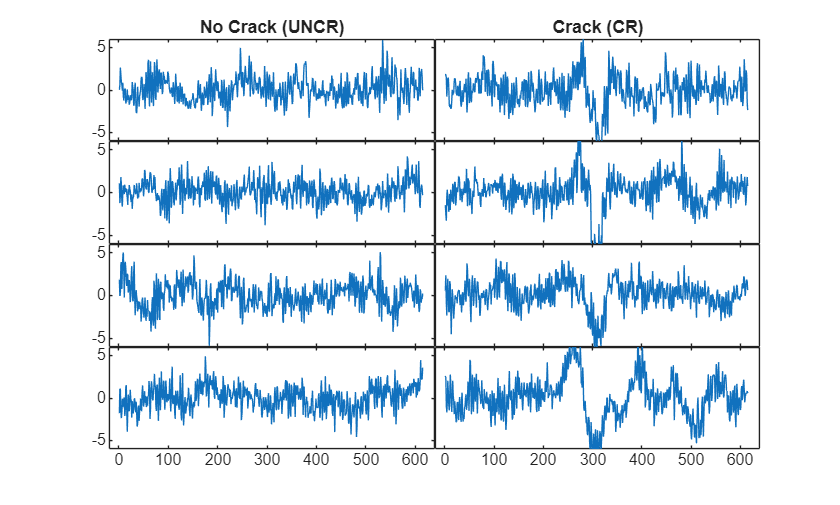
The signals indicate jolts where the vehicle drove over cracked sections of pavement. Each jolt is located at the center of the signal.

Preprocess Data

Next, partition the data into sets for training, validation, and testing. Partition the data into a training set containing 80% of the data, a validation set containing 10% of the data, and a test set containing the remaining 10% of the data. To partition the data, use the trainingPartitions function that is attached to this example as a supporting file. To access this file, open the example as a live script.

numObservations = numel(allroadData);
[idxTrain,idxValidation,idxTest] = trainingPartitions(numObservations,[0.8 0.1 0.1]);

XTrain = allroadData(idxTrain);
TTrain = allroadLabel(idxTrain);

XValidation = allroadData(idxValidation);
TValidation = allroadLabel(idxValidation);

XTest = allroadData(idxTest);
TTest = allroadLabel(idxTest);

Many deep learning techniques, including the compression techniques available in MATLAB®, require input data of uniform size. View the sequence lengths in allroadData.

tslen = cellfun(@length,allroadData);
figure
plot(tslen)
title("Sequence Length")

You can pad or truncate sequences to be the same length using the padsequences function. In this example, sequences that correspond to cracked pavement contain a sharp peak. If you truncate the sequences, then the peak can be truncated also. This truncation can negatively impact the quality of the model, so pad the sequences to be of equal length. Then, convert the sequences to dlarray objects.

XTrain = padsequences(XTrain,1,Direction="left");
XTrain = dlarray(XTrain,"TCB");

XValidation = padsequences(XValidation,1,Direction="left");
XValidation = dlarray(XValidation,"TCB");

XTest = padsequences(XTest,1,Direction="left");
XTest = dlarray(XTest,"TCB");

If your data does not fit into memory, then, instead of creating dlarray objects, you need to create a datastore containing your data and a minibatchqueue object to create and manage mini-batches of data for deep learning. For an example of creating a mini-batch queue for sequence classification, see Train Sequence Classification Network Using Custom Training Loop.

Next, transform the categorical labels into numerical arrays using the onehotencode function to facilitate compression later on. To train a classification network using trainnet, you can use the categorical labels without transforming them into numerical arrays.

labels = categories(allroadLabel);

TTrain = onehotencode(TTrain,2,ClassNames=labels);
TTrain = dlarray(TTrain,"BC");

TValidation = onehotencode(TValidation,2,ClassNames=labels);
TValidation = dlarray(TValidation,"BC");

TTest = onehotencode(TTest,2,ClassNames=labels);
TTest = dlarray(TTest,"BC");

Build and Train Network

Define the 1-D convolutional neural network architecture.

minLength = min(cellfun(@length,allroadData));
layers = [
    sequenceInputLayer(1,MinLength=minLength,Normalization="zerocenter")
    convolution1dLayer(3,16,Stride=2)
    batchNormalizationLayer
    reluLayer
    maxPooling1dLayer(4)
    convolution1dLayer(3,16,Padding="same")
    batchNormalizationLayer
    reluLayer
    maxPooling1dLayer(2)
    fullyConnectedLayer(32)
    reluLayer
    fullyConnectedLayer(2)
    globalAveragePooling1dLayer
    softmaxLayer
    ];

Specify these training options:

Train using the Adam optimizer.
Set the initial learn rate and learn rate schedule.
Train for a maximum of 200 epochs.
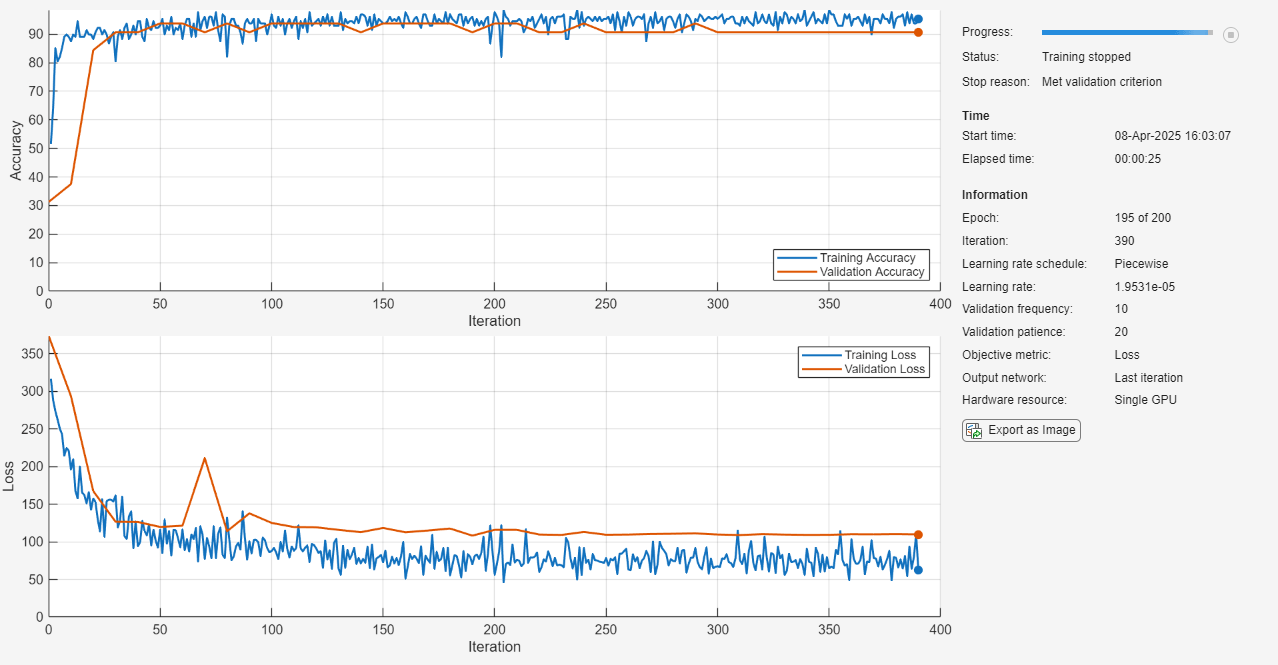
Display the training progress in a plot and disable the verbose output.
Specify the sequences and targets used for validation, validation patience, and frequency.
Return the network corresponding to the last training iteration.
Specify that the input data has the format "TCB" (time, channel, batch).
Shuffle the training data before each training epoch, and shuffle the validation data before each neural network validation.

options = trainingOptions("adam", ...
    InitialLearnRate=0.01, ...
    LearnRateSchedule="piecewise", ...
    LearnRateDropFactor=0.5, ...
    LearnRateDropPeriod=20, ...
    MaxEpochs=200, ...
    Verbose=false, ...
    Plots="training-progress", ...
    ValidationData={XValidation,TValidation}, ...
    ValidationPatience=20, ...
    ValidationFrequency=10, ...
    Metrics="accuracy", ...
    InputDataFormats="TCB", ...
    Shuffle="every-epoch", ...
    OutputNetwork="last-iteration");

The data is imbalanced, with twice as many sequences without pavement cracks than with pavement cracks.

nnz(allroadLabel=="CR")

ans = 
109

nnz(allroadLabel=="UNCR")

ans = 
218

Use a weighted classification loss with the class weights proportional to the inverse class frequencies. This loss prevents the network from achieving good results by classifying all sequences as uncracked.

numClasses = numel(labels);
for i=1:numClasses
    classFrequency(i) = nnz(allroadLabel == labels{i});
    classWeights(i) = numel(XTrain)/(numClasses*classFrequency(i));
end

lossFcn = @(Y,T) crossentropy(Y,T, ...
    classWeights, ...
    NormalizationFactor="all-elements", ...
    WeightsFormat="C") * numClasses;

For more information on working with imbalanced classes, see Train Sequence Classification Network Using Data with Imbalanced Classes.

Train the neural network using the trainnet function. Specify the custom loss function. By default, the trainnet function uses a GPU if one is available. Using a GPU requires a Parallel Computing Toolbox™ license and a supported GPU device. For information on supported devices, see GPU Computing Requirements (Parallel Computing Toolbox). Otherwise, the function uses the CPU. To specify the execution environment, use the ExecutionEnvironment training option.

netTrained = trainnet(XTrain,TTrain,layers,lossFcn,options);

Test Network

Test the neural network using the testnet function. For single-label classification, evaluate the accuracy. The accuracy is the percentage of correctly predicted labels. By default, the testnet function uses a GPU if one is available. To select the execution environment manually, use the ExecutionEnvironment argument of the testnet function.

testnet(netTrained,XTest,TTest,"accuracy")

ans = 
97.0588

Display the classification results in a confusion chart. Make predictions using the minibatchpredict function and convert the scores to labels using the onehotdecode function. By default, the minibatchpredict function uses a GPU if one is available.

YTest = minibatchpredict(netTrained,XTest);
YTestLabels = onehotdecode(YTest,labels,1);
TTestLabels = onehotdecode(TTest,labels,1);

Display the classification results in a confusion chart.

figure
confusionchart(TTestLabels,YTestLabels)

Save Network and Training Options

save("RoadDamageAnalysisNetwork","netTrained","options","idxTrain","idxValidation","idxTest","classWeights","numClasses")

In the next step in the workflow, you compress the network trained in this example using pruning, projection, and quantization to meet a fixed memory requirement.

Next step: Compress Sequence Classification Network for Road Damage Detection. You can also open the next example using the openExample function.

>> openExample('deeplearning_shared/CompressNetworkForRoadDamageDetectionExample')

References

[1] Yang, Qun, and Shishi Zhou. "Identification of Asphalt Pavement Transverse Cracking Based on Vehicle Vibration Signal Analysis." Road Materials and Pavement Design 22, no. 8 (August 3, 2021): 1780–98. https://doi.org/10.1080/14680629.2020.1714699.

[2] Zhou, Shishi. "Vehicle Vibration Data" 1 (September 5, 2019). https://doi.org/10.17632/3dvpjy4m22.1. Data is used under CC BY 4.0. Data is repackaged from original Excel data format to MAT files. Speed label removed and only "crack" or "nocrack" label retained.