msesim
Estimated mean squared error for adaptive filters
Syntax
Description
Examples
The mean squared error (MSE) measures the average of the squares of the errors between the desired signal and the primary signal input to the adaptive filter. Reducing this error converges the primary input to the desired signal. Determine the predicted value of MSE and the simulated value of MSE at each time instant using the msepred and msesim functions. Compare these MSE values with each other and with respect to the minimum MSE and steady-state MSE values. In addition, compute the sum of the squares of the coefficient errors given by the trace of the coefficient covariance matrix.
Initialization
Create a dsp.FIRFilter System object™ that represents the unknown system. Pass the signal, x, to the FIR filter. The output of the unknown system is the desired signal, d, which is the sum of the output of the unknown system (FIR filter) and an additive noise signal, n.
num = fir1(31,0.5);
fir = dsp.FIRFilter('Numerator',num);
iir = dsp.IIRFilter('Numerator',sqrt(0.75),...
        'Denominator',[1 -0.5]);
x = iir(sign(randn(2000,25)));
n = 0.1*randn(size(x));
d = fir(x) + n;
LMS Filter
Create a dsp.LMSFilter System object to create a filter that adapts to output the desired signal. Set the length of the adaptive filter to 32 taps, step size to 0.008, and the decimation factor for analysis and simulation to 5. The variable simmse represents the simulated MSE between the output of the unknown system, d, and the output of the adaptive filter. The variable mse gives the corresponding predicted value.
l = 32;
mu = 0.008;
m  = 5;

lms = dsp.LMSFilter('Length',l,'StepSize',mu);
[mmse,emse,meanW,mse,traceK] = msepred(lms,x,d,m);
[simmse,meanWsim,Wsim,traceKsim] = msesim(lms,x,d,m);
Plot the MSE Results
Compare the values of simulated MSE, predicted MSE, minimum MSE, and the final MSE. The final MSE value is given by the sum of minimum MSE and excess MSE.
nn = m:m:size(x,1);
semilogy(nn,simmse,[0 size(x,1)],[(emse+mmse)...
    (emse+mmse)],nn,mse,[0 size(x,1)],[mmse mmse])
title('Mean Squared Error Performance')
axis([0 size(x,1) 0.001 10])
legend('MSE (Sim.)','Final MSE','MSE','Min. MSE')
xlabel('Time Index')
ylabel('Squared Error Value')

The predicted MSE follows the same trajectory as the simulated MSE. Both these trajectories converge with the steady-state (final) MSE.
Plot the Coefficient Trajectories
meanWsim is the mean value of the simulated coefficients given by msesim. meanW is the mean value of the predicted coefficients given by msepred.
Compare the simulated and predicted mean values of LMS filter coefficients 12,13,14, and 15.
plot(nn,meanWsim(:,12),'b',nn,meanW(:,12),'r',nn,...
meanWsim(:,13:15),'b',nn,meanW(:,13:15),'r')
PlotTitle ={'Average Coefficient Trajectories for';...
            'W(12), W(13), W(14), and W(15)'}
PlotTitle = 2×1 cell
    {'Average Coefficient Trajectories for'}
    {'W(12), W(13), W(14), and W(15)'      }
title(PlotTitle)
legend('Simulation','Theory')
xlabel('Time Index')
ylabel('Coefficient Value')

In steady state, both the trajectories converge.
Sum of Squared Coefficient Errors
Compare the sum of the squared coefficient errors given by msepred and msesim. These values are given by the trace of the coefficient covariance matrix.
semilogy(nn,traceKsim,nn,traceK,'r')
title('Sum-of-Squared Coefficient Errors')
axis([0 size(x,1) 0.0001 1])
legend('Simulation','Theory')
xlabel('Time Index')
ylabel('Squared Error Value')

Identify an unknown system by performing active noise control using a filtered-x LMS algorithm. The objective of the adaptive filter is to minimize the error signal between the output of the adaptive filter and the output of the unknown system (or the system to be identified). Once the error signal is minimal, the unknown system converges to the adaptive filter.
Initialization
Create a dsp.FIRFilter System object that represents the system to be identified. Pass the signal, x, to the FIR filter. The output of the unknown system is the desired signal, d, which is the sum of the output of the unknown system (FIR filter) and an additive noise signal, n.
num = fir1(31,0.5);
fir = dsp.FIRFilter(Numerator=num);
iir = dsp.IIRFilter(Numerator=sqrt(0.75),...
        Denominator=[1 -0.5]);
x = iir(sign(randn(2000,25)));
n = 0.1*randn(size(x));
d = fir(x) + n;
Adaptive Filter
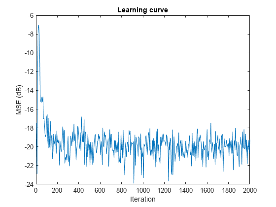
Create a dsp.FilteredXLMSFilter System object to create an adaptive filter that uses the filtered-x LMS algorithm. Set the length of the adaptive filter to 32 taps, step size to 0.008, and the decimation factor for analysis and simulation to 5. The variable simmse represents the error between the output of the unknown system, d, and the output of the adaptive filter.
l = 32;
mu = 0.008;
m  = 5;
fxlms = dsp.FilteredXLMSFilter(l,StepSize=mu);
[simmse,meanWsim,Wsim,traceKsim] = msesim(fxlms,x,d,m);
plot(m*(1:length(simmse)),10*log10(simmse))
xlabel("Iteration")
ylabel("MSE (dB)")
% Plot the learning curve for filtered-x LMS filter
% used in system identification
title("Learning curve")

With each iteration of adaptation, the value of simmse decreases to a minimal value, indicating that the unknown system has converged to the adaptive filter.
ha = fir1(31,0.5);
% FIR system to be identified
fir = dsp.FIRFilter(Numerator=ha);
iir = dsp.IIRFilter(Numerator=sqrt(0.75),...
        Denominator=[1 -0.5]);
x = iir(sign(randn(2000,25)));
% Observation noise signal
n = 0.1*randn(size(x));
 % Desired signal
d = fir(x)+n;
% Filter length
l = 32;
% Decimation factor for analysis
% and simulation results
m  = 5;
ha = dsp.AdaptiveLatticeFilter(l);
[simmse,meanWsim,Wsim,traceKsim] = msesim(ha,x,d,m);
plot(m*(1:length(simmse)),10*log10(simmse));
xlabel("Iteration");
ylabel("MSE (dB)");
% Plot the learning curve used for
% adaptive lattice filter used in system identification
title("Learning Curve")

fir = fir1(31,0.5);
% FIR system to be identified
firFilter = dsp.FIRFilter(Numerator=fir);
iirFilter = dsp.IIRFilter(Numerator=sqrt(0.75),...
        Denominator=[1 -0.5]);
x = iirFilter(sign(randn(2000,25)));
% Observation noise signal
n = 0.1*randn(size(x));
% Desired signal
d = firFilter(x)+n;
% Filter length
l = 32;
% Block LMS Step size
mu = 0.008;
% Decimation factor for analysis
% and simulation results
m  = 32;
fir = dsp.BlockLMSFilter(l,StepSize=mu);
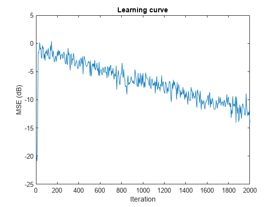
[simmse,meanWsim,Wsim,traceKsim] = msesim(fir,x,d,m);
plot(m*(1:length(simmse)),10*log10(simmse));
xlabel("Iteration"); ylabel("MSE (dB)");
% Plot the learning curve for
% block LMS filter used in system identification
title("Learning curve")

ha = fir1(31,0.5);
% FIR system to be identified
fir = dsp.FIRFilter(Numerator=ha);
iir = dsp.IIRFilter(Numerator=sqrt(0.75),...
        Denominator=[1 -0.5]);
x = iir(sign(randn(2000,25)));
% Observation noise signal
n = 0.1*randn(size(x));
% Desired signal
d = fir(x)+n;
% Filter length
l = 32;
% Affine Projection filter Step size.
mu = 0.008;
% Decimation factor for analysis
% and simulation results
m  = 5;

apf = dsp.AffineProjectionFilter(l,"StepSize",mu);
[simmse,meanWsim,Wsim,traceKsim] = msesim(apf,x,d,m);
plot(m*(1:length(simmse)),10*log10(simmse));
xlabel("Iteration"); ylabel("MSE (dB)");
% Plot the learning curve for affine projection filter
% used in system identification
title("Learning Curve")

Input Arguments
Adaptive filter, specified as one of the following System objects:
Input signal, specified as a scalar, column vector, or matrix. Columns of
the matrix x contain individual input signal sequences.
The input, x, and the desired signal,
d, must have the same size and data type.
If adaptFilt is a dsp.BlockLMSFilter object, the
input signal frame size must be greater than or equal to the value you
specify in the BlockSize property of the object.
Data Types: single | double
Desired response signal, specified as a scalar, column vector, or matrix.
Columns of the matrix d contain individual desired
signal sequences. The input, x, and the desired signal,
d, must have the same size and the data
type.
If adaptFilt is a dsp.BlockLMSFilter
System object, the desired signal frame size must be greater than or equal
to the value you specify in the BlockSize property of
the object.
Data Types: single | double
Decimation factor, specified as a positive scalar. Every
mth value of the estimated sequences is saved into
the corresponding output arguments, mse,
meanw, w, and
tracek. If m equals 1, every
value of these sequences is saved.
If adaptFilt is a dsp.BlockLMSFilter
System object, the decimation factor must be a multiple of the value you
specify in the BlockSize property of the object.
Data Types: single | double | int8 | int16 | int32 | int64 | uint8 | uint16 | uint32 | uint64 | logical
Output Arguments
Estimates of the mean squared error of the adaptive filter at each time instant, returned as a column vector.
If the adaptive filter is dsp.BlockLMSFilter and the
decimation factor m is specified, length of
mse equals floor(M/m).
M is the frame size (number of rows) of the input
signal, x. If m is not specified,
the length of mse equals floor(M/B),
where B is the value you specify in the
BlockSize property of the object. The input signal
frame size must be greater than or equal to the value you specify in the
BlockSize property of the object. The decimation
factor, if specified, must be a multiple of the
BlockSize property.
For the other adaptive filters, if the decimation factor,
m = 1, the length of mse
equals the frame size of the input signal. If m > 1,
the length of mse equals
floor(M/m).
Data Types: double
Sequence of coefficient vector means of the adaptive filter at each time instant, estimated as a matrix. The columns of this matrix contain estimates of the mean values of the adaptive filter coefficients at each time instant.
If the adaptive filter is dsp.BlockLMSFilter and the
decimation factor m is specified, the dimensions of
meanw is
floor(M/m)-by-N.
M is the frame size (number of rows) of the input
signal, x. N is the length of the
filter weights vector, specified by the Length property
of the adaptive filter. If m is not specified, the
dimensions of meanw is
floor(M/B)-by-N, where
B is the value you specify in the
BlockSize property of the object. The input signal
frame size must be greater than or equal to the value you specify in the
BlockSize property of the object. The decimation
factor, if specified, must be a multiple of the
BlockSize property.
For the other adaptive filters, If the decimation factor,
m = 1, the dimensions of meanw
is M-by-N. If m >
1, the dimensions of meanw is
floor(M/m)-by-N.
Data Types: double
Final values of the adaptive filter coefficients for the algorithm
corresponding to adaptFilt, returned as a row vector. The
length of the row vector equals the value you specify in the
Length property of the object.
Data Types: single | double
Sequence of total coefficient error powers, estimated as a column vector. This column vector contains estimates of the total coefficient error power of the adaptive filter at each time instant.
If the adaptive filter is dsp.BlockLMSFilter and the
decimation factor m is specified, length of
tracek equals floor(M/m).
M is the frame size (number of rows) of the input
signal, x. If m is not specified,
the length of tracek equals
floor(M/B), where B is the value
you specify in the BlockSize property of the object.
The input signal frame size must be greater than or equal to the value you
specify in the BlockSize property of the object. The
decimation factor, if specified, must be a multiple of the
BlockSize property.
For the other adaptive filters, if the decimation factor,
m = 1, the length of tracek
equals the frame size of the input signal. If m > 1,
the length of tracek equals
floor(M/m).
Data Types: double
References
[1] Hayes, M.H. Statistical Digital Signal Processing and Modeling. New York: John Wiley & Sons, 1996.
Version History
Introduced in R2012a
See Also
Functions
Objects
MATLAB Command
You clicked a link that corresponds to this MATLAB command:
Run the command by entering it in the MATLAB Command Window. Web browsers do not support MATLAB commands.
Seleccione un país/idioma
Seleccione un país/idioma para obtener contenido traducido, si está disponible, y ver eventos y ofertas de productos y servicios locales. Según su ubicación geográfica, recomendamos que seleccione: .
También puede seleccionar uno de estos países/idiomas:
Cómo obtener el mejor rendimiento
Seleccione China (en idioma chino o inglés) para obtener el mejor rendimiento. Los sitios web de otros países no están optimizados para ser accedidos desde su ubicación geográfica.
América
- América Latina (Español)
- Canada (English)
- United States (English)
Europa
- Belgium (English)
- Denmark (English)
- Deutschland (Deutsch)
- España (Español)
- Finland (English)
- France (Français)
- Ireland (English)
- Italia (Italiano)
- Luxembourg (English)
- Netherlands (English)
- Norway (English)
- Österreich (Deutsch)
- Portugal (English)
- Sweden (English)
- Switzerland
- United Kingdom (English)