simulate
Simulate regression coefficients and disturbance variance of Bayesian linear regression model
Syntax
Description
[
returns a random vector of regression coefficients (BetaSim,sigma2Sim]
= simulate(Mdl)BetaSim)
and a random disturbance variance (sigma2Sim) drawn from the
Bayesian linear regression
model
Mdl of β and
σ2.
[
draws from the marginal posterior distributions produced or updated by
incorporating the predictor data BetaSim,sigma2Sim]
= simulate(Mdl,X,y)X and corresponding response
data y.
If
Mdlis a joint prior model, thensimulateproduces the marginal posterior distributions by updating the prior model with information about the parameters that it obtains from the data.If
Mdlis a marginal posterior model, thensimulateupdates the posteriors with information about the parameters that it obtains from the additional data. The complete data likelihood is composed of the additional dataXandy, and the data that createdMdl.
NaNs in the data indicate missing values, which
simulate removes by using list-wise deletion.
[
uses any of the input argument combinations in the previous syntaxes and
additional options specified by one or more name-value pair arguments. For
example, you can specify a value for β or
σ2 to simulate from the
conditional posterior distribution of one parameter,
given the specified value of the other parameter.BetaSim,sigma2Sim]
= simulate(___,Name,Value)
[
also returns draws from the latent regime distribution if BetaSim,sigma2Sim,RegimeSim]
= simulate(___)Mdl
is a Bayesian linear regression model for stochastic search variable selection
(SSVS), that is, if Mdl is a mixconjugateblm or mixsemiconjugateblm model object.
Examples
Consider the multiple linear regression model that predicts the US real gross national product (GNPR) by using a linear combination of industrial production index (IPI), total employment (E), and real wages (WR).
For all , is a series of independent Gaussian disturbances with a mean of 0 and variance .
Assume these prior distributions:
. is a 4-by-1 vector of means, and is a scaled 4-by-4 positive definite covariance matrix.
. and are the shape and scale, respectively, of an inverse gamma distribution.
These assumptions and the data likelihood imply a normal-inverse-gamma conjugate model.
Load the Nelson-Plosser data set. Create variables for the response and predictor series.
load Data_NelsonPlosser
varNames = {'IPI' 'E' 'WR'};
X = DataTable{:,varNames};
y = DataTable{:,'GNPR'};
Create a normal-inverse-gamma conjugate prior model for the linear regression parameters. Specify the number of predictors p and the variable names.
p = 3;
PriorMdl = bayeslm(p,'ModelType','conjugate','VarNames',varNames);
PriorMdl is a conjugateblm Bayesian linear regression model object representing the prior distribution of the regression coefficients and disturbance variance.
Simulate a set of regression coefficients and a value of the disturbance variance from the prior distribution.
rng(1); % For reproducibility
[betaSimPrior,sigma2SimPrior] = simulate(PriorMdl)
betaSimPrior = 4×1
-33.5917
-49.1445
-37.4492
-25.3632
sigma2SimPrior =
0.1962
betaSimPrior is the randomly drawn 4-by-1 vector of regression coefficients corresponding to the names in PriorMdl.VarNames. The sigma2SimPrior output is the randomly drawn scalar disturbance variance.
Estimate the posterior distribution.
PosteriorMdl = estimate(PriorMdl,X,y);
Method: Analytic posterior distributions
Number of observations: 62
Number of predictors:   4
Log marginal likelihood: -259.348

           |   Mean      Std          CI95        Positive       Distribution
-----------------------------------------------------------------------------------
 Intercept | -24.2494  8.7821  [-41.514, -6.985]    0.003   t (-24.25, 8.65^2, 68)
 IPI       |   4.3913  0.1414   [ 4.113,  4.669]    1.000   t (4.39, 0.14^2, 68)
 E         |   0.0011  0.0003   [ 0.000,  0.002]    1.000   t (0.00, 0.00^2, 68)
 WR        |   2.4683  0.3490   [ 1.782,  3.154]    1.000   t (2.47, 0.34^2, 68)
 Sigma2    |  44.1347  7.8020   [31.427, 61.855]    1.000   IG(34.00, 0.00069)
PosteriorMdl is a conjugateblm Bayesian linear regression model object representing the posterior distribution of the regression coefficients and disturbance variance.
Simulate a set of regression coefficients and a value of the disturbance variance from the posterior distribution.
[betaSimPost,sigma2SimPost] = simulate(PosteriorMdl)
betaSimPost = 4×1

  -25.9351
    4.4379
    0.0012
    2.4072
sigma2SimPost =
41.9575
betaSimPost and sigma2SimPost have the same dimensions as betaSimPrior and sigma2SimPrior, respectively, but are drawn from the posterior.
Consider the regression model in Simulate Parameter Value from Prior and Posterior Distributions.
Load the data and create a conjugate prior model for the regression coefficients and the disturbance variance. Then, estimate the posterior distribution and return the estimation summary table.
load Data_NelsonPlosser
varNames = {'IPI' 'E' 'WR'};
X = DataTable{:,varNames};
y = DataTable{:,'GNPR'};
p = 3;
PriorMdl = bayeslm(p,'ModelType','conjugate','VarNames',varNames);
[PosteriorMdl,Summary] = estimate(PriorMdl,X,y);
Method: Analytic posterior distributions
Number of observations: 62
Number of predictors:   4
Log marginal likelihood: -259.348

           |   Mean      Std          CI95        Positive       Distribution
-----------------------------------------------------------------------------------
 Intercept | -24.2494  8.7821  [-41.514, -6.985]    0.003   t (-24.25, 8.65^2, 68)
 IPI       |   4.3913  0.1414   [ 4.113,  4.669]    1.000   t (4.39, 0.14^2, 68)
 E         |   0.0011  0.0003   [ 0.000,  0.002]    1.000   t (0.00, 0.00^2, 68)
 WR        |   2.4683  0.3490   [ 1.782,  3.154]    1.000   t (2.47, 0.34^2, 68)
 Sigma2    |  44.1347  7.8020   [31.427, 61.855]    1.000   IG(34.00, 0.00069)
Summary is a table containing the statistics that estimate displays at the command line.
Although the marginal and conditional posterior distributions of and are analytically tractable, this example focuses on how to implement the Gibbs sampler to reproduce known results.
Estimate the model again, but use a Gibbs sampler. Alternate between sampling from the conditional posterior distributions of the parameters. Sample 10,000 times and create variables for preallocation. Start the sampler by drawing from the conditional posterior of given .
m = 1e4;
BetaDraws = zeros(p + 1,m);
sigma2Draws = zeros(1,m + 1);
sigma2Draws(1) = 2;
rng(1); % For reproducibility
for j = 1:m
    BetaDraws(:,j) = simulate(PriorMdl,X,y,'Sigma2',sigma2Draws(j));
    [~,sigma2Draws(j + 1)] = simulate(PriorMdl,X,y,'Beta',BetaDraws(:,j));
end
sigma2Draws = sigma2Draws(2:end); % Remove initial value from MCMC sample
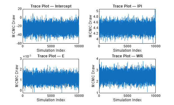
Graph trace plots of the parameters.
figure;
for j = 1:(p + 1);
    subplot(2,2,j);
    plot(BetaDraws(j,:))
    ylabel('MCMC Draw')
    xlabel('Simulation Index')
    title(sprintf('Trace Plot — %s',PriorMdl.VarNames{j}));
end
figure;
plot(sigma2Draws)
ylabel('MCMC Draw')
xlabel('Simulation Index')
title('Trace plot — Sigma2')
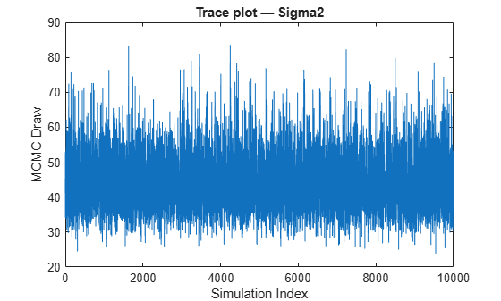
The Markov chain Monte Carlo (MCMC) samples appear to converge and mix well.
Apply a burn-in period of 1000 draws, and then compute the means and standard deviations of the MCMC samples. Compare them with the estimates from estimate.
bp = 1000;
postBetaMean = mean(BetaDraws(:,(bp + 1):end),2);
postSigma2Mean = mean(sigma2Draws(:,(bp + 1):end));
postBetaStd = std(BetaDraws(:,(bp + 1):end),[],2);
postSigma2Std = std(sigma2Draws((bp + 1):end));
[Summary(:,1:2),table([postBetaMean; postSigma2Mean],...
    [postBetaStd; postSigma2Std],'VariableNames',{'GibbsMean','GibbsStd'})]
ans=5×4 table
                   Mean          Std        GibbsMean     GibbsStd
                 _________    __________    _________    __________

    Intercept      -24.249        8.7821      -24.293         8.748
    IPI             4.3913        0.1414       4.3917       0.13941
    E            0.0011202    0.00032931    0.0011229    0.00032875
    WR              2.4683       0.34895       2.4654       0.34364
    Sigma2          44.135         7.802       44.011        7.7816
The estimates are very close. MCMC variations account for the differences.
Consider the regression model in Simulate Parameter Value from Prior and Posterior Distributions.
Assume these prior distributions for = 0,...,3:
, where and are independent, standard normal random variables. Therefore, the coefficients have a Gaussian mixture distribution. Assume all coefficients are conditionally independent, a priori, but they are dependent on the disturbance variance.
. and are the shape and scale, respectively, of an inverse gamma distribution.
and it represents the random variable-inclusion regime variable with a discrete uniform distribution.
Create a prior model for performing SSVS. Assume that and are dependent (a conjugate mixture model). Specify the number of predictors p and the names of the regression coefficients.
p = 3;
PriorMdl = mixconjugateblm(p,'VarNames',["IPI" "E" "WR"]);
Load the Nelson-Plosser data set. Create variables for the response and predictor series.
load Data_NelsonPlosser
X = DataTable{:,PriorMdl.VarNames(2:end)};
y = DataTable{:,'GNPR'};
Compute the number of possible regimes, that is, number of combinations that result from including and excluding variables in the model.
cardRegime = 2^(PriorMdl.Intercept + PriorMdl.NumPredictors)
cardRegime =
16
Simulate 10,000 regimes from the posterior distribution.
rng(1);
[~,~,RegimeSim] = simulate(PriorMdl,X,y,'NumDraws',10000);
RegimeSim is a 4-by-1000 logical matrix. Rows correspond to the variables in Mdl.VarNames, and columns correspond to draws from the posterior distribution.
Plot a histogram of the regimes visited. Recode the regimes so that they are readable. Specifically, for each regime, create a string that identifies the variables in the model, and separate the variables with dots.
cRegime = num2cell(RegimeSim,1);
cRegime = categorical(cellfun(@(c)join(PriorMdl.VarNames(c),"."),cRegime));
cRegime(ismissing(cRegime)) = "NoCoefficients";

histogram(cRegime);
title('Variables Included in Models')
ylabel('Frequency');
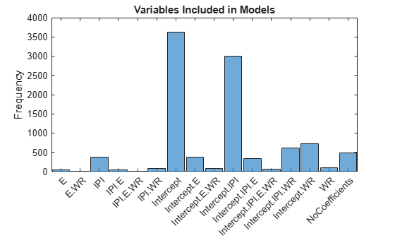
Compute the marginal posterior probability of variable inclusion.
table(mean(RegimeSim,2),'RowNames',PriorMdl.VarNames,...
    'VariableNames',"Regime")
ans=4×1 table
                 Regime
                 ______

    Intercept    0.8829
    IPI          0.4547
    E             0.098
    WR           0.1692
Consider a Bayesian linear regression model containing one predictor, and a t distributed disturbance variance with a profiled degrees of freedom parameter .
.
These assumptions imply:
is a vector of latent scale parameters that attributes low precision to observations far from the regression line. is a hyperparameter controlling the influence of on the observations.
For this problem, the Gibbs sampler is well suited to estimate the coefficients because you can simulate the parameters of a Bayesian linear regression model conditioned on , and then simulate from its conditional distribution.
Generate responses from where and .
rng('default');
n = 100;
x = linspace(0,2,n)';
b0 = 1;
b1 = 2;
sigma = 0.5;
e = randn(n,1);
y = b0 + b1*x + sigma*e;
Introduce outlying responses by inflating all responses below by a factor of 3.
y(x < 0.25) = y(x < 0.25)*3;
Fit a linear model to the data. Plot the data and the fitted regression line.
Mdl = fitlm(x,y)
Mdl =
Linear regression model:
    y ~ 1 + x1

Estimated Coefficients:
                   Estimate      SE       tStat       pValue
                   ________    _______    ______    __________

    (Intercept)     2.6814     0.28433    9.4304    2.0859e-15
    x1             0.78974     0.24562    3.2153     0.0017653


Number of observations: 100, Error degrees of freedom: 98
Root Mean Squared Error: 1.43
R-squared: 0.0954,  Adjusted R-Squared: 0.0862
F-statistic vs. constant model: 10.3, p-value = 0.00177
figure;
plot(Mdl);
hl = legend;
hold on;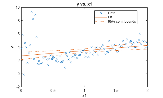
The simulated outliers appear to influence the fitted regression line.
Implement this Gibbs sampler:
Draw parameters from the posterior distribution of . Deflate the observations by , create a diffuse prior model with two regression coefficients, and draw a set of parameters from the posterior. The first regression coefficient corresponds to the intercept, so specify that
bayeslmnot include an intercept.Compute residuals.
Draw values from the conditional posterior of .
Run the Gibbs sampler for 20,000 iterations and apply a burn-in period of 5,000. Specify , preallocate for the posterior draws, and initialize to a vector of ones.
m = 20000;
nu = 1;
burnin = 5000;
lambda = ones(n,m + 1);
estBeta = zeros(2,m + 1);
estSigma2 = zeros(1,m + 1);
for j = 1:m
    yDef = y./sqrt(lambda(:,j));
    xDef = [ones(n,1) x]./sqrt(lambda(:,j));
    PriorMdl = bayeslm(2,'Model','diffuse','Intercept',false);
    [estBeta(:,j + 1),estSigma2(1,j + 1)] = simulate(PriorMdl,xDef,yDef);
    ep = y - [ones(n,1) x]*estBeta(:,j + 1);
    sp = (nu + 1)/2;
    sc =  2./(nu + ep.^2/estSigma2(1,j + 1));
    lambda(:,j + 1) = 1./gamrnd(sp,sc);
end
A good practice is to diagnose the MCMC sampler by examining trace plots. For brevity, this example skips this task.
Compute the mean of the draws from the posterior of the regression coefficients. Remove the burn-in period draws.
postEstBeta = mean(estBeta(:,(burnin + 1):end),2)
postEstBeta = 2×1

    1.3971
    1.7051
The estimate of the intercept is lower and the slope is higher than the estimates returned by fitlm.
Plot the robust regression line with the regression line fitted by least squares.
h = gca;
xlim = h.XLim';
plotY = [ones(2,1) xlim]*postEstBeta;
plot(xlim,plotY,'LineWidth',2);
hl.String{4} = 'Robust Bayes';
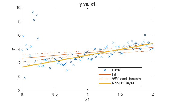
The regression line fit using robust Bayesian regression appears to be a better fit.
The maximum a posteriori probability (MAP) estimate is the posterior mode, that is, the parameter value that yields the maximum of the posterior pdf. If the posterior is analytically intractable, then you can use Monte Carlo sampling to estimate the MAP.
Consider the linear regression model in Simulate Parameter Value from Prior and Posterior Distributions.
Load the Nelson-Plosser data set. Create variables for the response and predictor series.
load Data_NelsonPlosser
varNames = {'IPI' 'E' 'WR'};
X = DataTable{:,varNames};
y = DataTable{:,'GNPR'};
Create a normal-inverse-gamma conjugate prior model for the linear regression parameters. Specify the number of predictors p and the variable names.
p = 3;
PriorMdl = bayeslm(p,'ModelType','conjugate','VarNames',varNames)
PriorMdl =
  conjugateblm with properties:

    NumPredictors: 3
        Intercept: 1
         VarNames: {4×1 cell}
               Mu: [4×1 double]
                V: [4×4 double]
                A: 3
                B: 1


           |  Mean     Std            CI95         Positive       Distribution
-----------------------------------------------------------------------------------
 Intercept |  0      70.7107  [-141.273, 141.273]    0.500   t (0.00, 57.74^2,  6)
 IPI       |  0      70.7107  [-141.273, 141.273]    0.500   t (0.00, 57.74^2,  6)
 E         |  0      70.7107  [-141.273, 141.273]    0.500   t (0.00, 57.74^2,  6)
 WR        |  0      70.7107  [-141.273, 141.273]    0.500   t (0.00, 57.74^2,  6)
 Sigma2    | 0.5000   0.5000    [ 0.138,  1.616]     1.000   IG(3.00,    1)
Estimate the marginal posterior distributions of and .
rng(1); % For reproducibility
PosteriorMdl = estimate(PriorMdl,X,y);
Method: Analytic posterior distributions
Number of observations: 62
Number of predictors: 4
Log marginal likelihood: -259.348
| Mean Std CI95 Positive Distribution
-----------------------------------------------------------------------------------
Intercept | -24.2494 8.7821 [-41.514, -6.985] 0.003 t (-24.25, 8.65^2, 68)
IPI | 4.3913 0.1414 [ 4.113, 4.669] 1.000 t (4.39, 0.14^2, 68)
E | 0.0011 0.0003 [ 0.000, 0.002] 1.000 t (0.00, 0.00^2, 68)
WR | 2.4683 0.3490 [ 1.782, 3.154] 1.000 t (2.47, 0.34^2, 68)
Sigma2 | 44.1347 7.8020 [31.427, 61.855] 1.000 IG(34.00, 0.00069)
The display includes the marginal posterior distribution statistics.
Extract the posterior mean of from the posterior model, and extract the posterior covariance of from the estimation summary returned by summarize.
estBetaMean = PosteriorMdl.Mu;
Summary = summarize(PosteriorMdl);
EstBetaCov = Summary.Covariances{1:(end - 1),1:(end - 1)};
estBetaMean is a 4-by-1 vector representing the mean of the marginal posterior of . EstBetaCov is a 4-by-4 matrix representing the covariance matrix of the posterior of .
Draw 10,000 parameter values from the posterior distribution.
rng(1); % For reproducibility
[BetaSim,sigma2Sim] = simulate(PosteriorMdl,'NumDraws',1e5);
BetaSim is a 4-by-10,000 matrix of randomly drawn regression coefficients. sigma2Sim is a 1-by-10,000 vector of randomly drawn disturbance variances.
Transpose and standardize the matrix of regression coefficients. Compute the correlation matrix of the regression coefficients.
estBetaStd = sqrt(diag(EstBetaCov)');
BetaSim = BetaSim';
BetaSimStd = (BetaSim - estBetaMean')./estBetaStd;
BetaCorr = corrcov(EstBetaCov);
BetaCorr = (BetaCorr + BetaCorr')/2; % Enforce symmetry
Because the marginal posterior distributions are known, evaluate the posterior pdf at all simulated values.
betaPDF = mvtpdf(BetaSimStd,BetaCorr,68);
a = 34;
b = 0.00069;
igPDF = @(x,ap,bp)1./(gamma(ap).*bp.^ap).*x.^(-ap-1).*exp(-1./(x.*bp));...
    % Inverse gamma pdf
sigma2PDF = igPDF(sigma2Sim,a,b);
Find the simulated values that maximize the respective pdfs, that is, the posterior modes.
[~,idxMAPBeta] = max(betaPDF);
[~,idxMAPSigma2] = max(sigma2PDF);
betaMAP = BetaSim(idxMAPBeta,:);
sigma2MAP = sigma2Sim(idxMAPSigma2);
betaMAP and sigma2MAP are the MAP estimates.
Because the posterior of is symmetric and unimodal, the posterior mean and MAP should be the same. Compare the MAP estimate of with its posterior mean.
table(betaMAP',PosteriorMdl.Mu,'VariableNames',{'MAP','Mean'},...
    'RowNames',PriorMdl.VarNames)
ans=4×2 table
                    MAP         Mean
                 _________    _________

    Intercept      -24.559      -24.249
    IPI             4.3964       4.3913
    E            0.0011389    0.0011202
    WR              2.4473       2.4683
The estimates are fairly close to one another.
Estimate the analytical mode of the posterior of . Compare it to the estimated MAP of .
igMode = 1/(b*(a+1))
igMode =
41.4079
sigma2MAP
sigma2MAP =
41.4075
These estimates are also fairly close.
Input Arguments
Name-Value Arguments
Output Arguments
Limitations
simulatecannot draw values from an improper distribution, that is, a distribution whose density does not integrate to 1.If
Mdlis anempiricalblmmodel object, then you cannot specifyBetaorSigma2. You cannot simulate from the conditional posterior distributions by using an empirical distribution.
More About
Algorithms
Whenever
simulatemust estimate a posterior distribution (for example, whenMdlrepresents a prior distribution and you supplyXandy) and the posterior is analytically tractable,simulatesimulates directly from the posterior. Otherwise,simulateresorts to Monte Carlo simulation to estimate the posterior. For more details, see Posterior Estimation and Inference.If
Mdlis a joint posterior model, thensimulatesimulates data from it differently compared to whenMdlis a joint prior model and you supplyXandy. Therefore, if you set the same random seed and generate random values both ways, then you might not obtain the same values. However, corresponding empirical distributions based on a sufficient number of draws is effectively equivalent.This figure shows how
simulatereduces the sample by using the values ofNumDraws,Thin, andBurnIn.
Rectangles represent successive draws from the distribution.
simulateremoves the white rectangles from the sample. The remainingNumDrawsblack rectangles compose the sample.If
Mdlis asemiconjugateblmmodel object, thensimulatesamples from the posterior distribution by applying the Gibbs sampler.simulateuses the default value ofSigma2Startfor σ2 and draws a value of β from π(β|σ2,X,y).simulatedraws a value of σ2 from π(σ2|β,X,y) by using the previously generated value of β.The function repeats steps 1 and 2 until convergence. To assess convergence, draw a trace plot of the sample.
If you specify
BetaStart, thensimulatedraws a value of σ2 from π(σ2|β,X,y) to start the Gibbs sampler.simulatedoes not return this generated value of σ2.If
Mdlis anempiricalblmmodel object and you do not supplyXandy, thensimulatedraws fromMdl.BetaDrawsandMdl.Sigma2Draws. IfNumDrawsis less than or equal tonumel(Mdl.Sigma2Draws), thensimulatereturns the firstNumDrawselements ofMdl.BetaDrawsandMdl.Sigma2Drawsas random draws for the corresponding parameter. Otherwise,simulaterandomly resamplesNumDrawselements fromMdl.BetaDrawsandMdl.Sigma2Draws.If
Mdlis acustomblmmodel object, thensimulateuses an MCMC sampler to draw from the posterior distribution. At each iteration, the software concatenates the current values of the regression coefficients and disturbance variance into an (Mdl.Intercept+Mdl.NumPredictors+ 1)-by-1 vector, and passes it toMdl.LogPDF. The value of the disturbance variance is the last element of this vector.The HMC sampler requires both the log density and its gradient. The gradient should be a
(NumPredictors+Intercept+1)-by-1 vector. If the derivatives of certain parameters are difficult to compute, then, in the corresponding locations of the gradient, supplyNaNvalues instead.simulatereplacesNaNvalues with numerical derivatives.If
Mdlis alassoblm,mixconjugateblm, ormixsemiconjugateblmmodel object and you supplyXandy, thensimulatesamples from the posterior distribution by applying the Gibbs sampler. If you do not supply the data, thensimulatesamples from the analytical, unconditional prior distributions.simulatedoes not return default starting values that it generates.If
Mdlis amixconjugateblmormixsemiconjugateblm, thensimulatedraws from the regime distribution first, given the current state of the chain (the values ofRegimeStart,BetaStart, andSigma2Start). If you draw one sample and do not specify values forRegimeStart,BetaStart, andSigma2Start, thensimulateuses the default values and issues a warning.
Version History
Introduced in R2017a
See Also
Objects
conjugateblm|customblm|empiricalblm|semiconjugateblm|diffuseblm|mixconjugateblm|mixsemiconjugateblm|lassoblm