Evaluate Quality Metrics on eSFR Test Chart
This example shows how to perform standard quality measurements on an Imatest® edge spatial frequency response (eSFR) test chart. Measured properties include sharpness, chromatic aberration, noise, illumination, and color accuracy.
Create a Test Chart Object
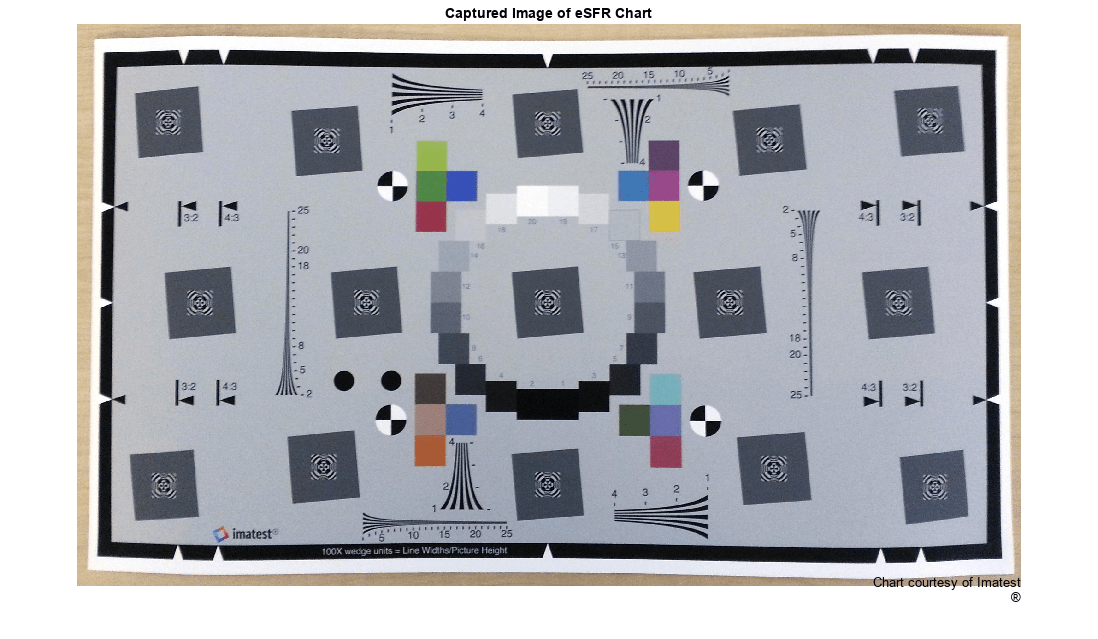
Read an image of an eSFR chart into the workspace. Display the chart.
I = imread("eSFRTestImage.jpg");
imshow(I)
title("Captured Image of eSFR Chart")
text(size(I,2),size(I,1)+15,["Chart courtesy of Imatest",char(174)], ...
    FontSize=10,HorizontalAlignment="right");
Create an eSFR test chart object that automatically defines regions of interest (ROIs) based on detected registration markers.
chart = esfrChart(I);
Highlight and label the detected ROIs to visually confirm that the ROIs are suitable for measurements.
displayChart(chart)
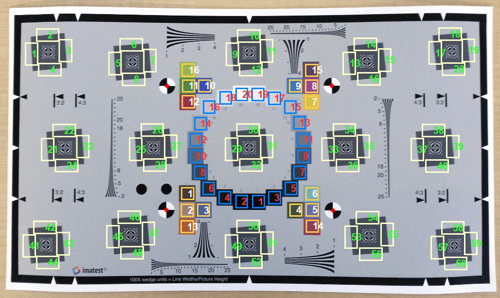
All 60 slanted edge ROIs (labeled in green) are visible and centered on appropriate edges. In addition, 20 gray patch ROIs (labeled in red) and 16 color patch ROIs (labeled in white) are visible and are contained within the boundary of each patch. The chart is correctly imported.
Measure Edge Sharpness
Measure the sharpness of all 60 slanted edge ROIs. Also measure the averaged horizontal and vertical sharpness of these ROIs.
[sharpnessTable,aggregateSharpnessTable] = measureSharpness(chart);
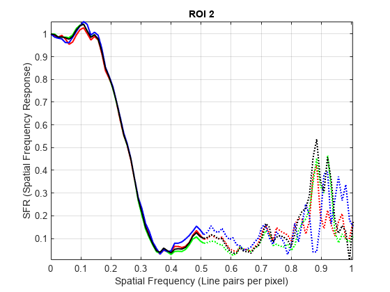
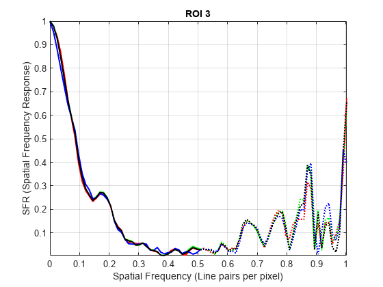
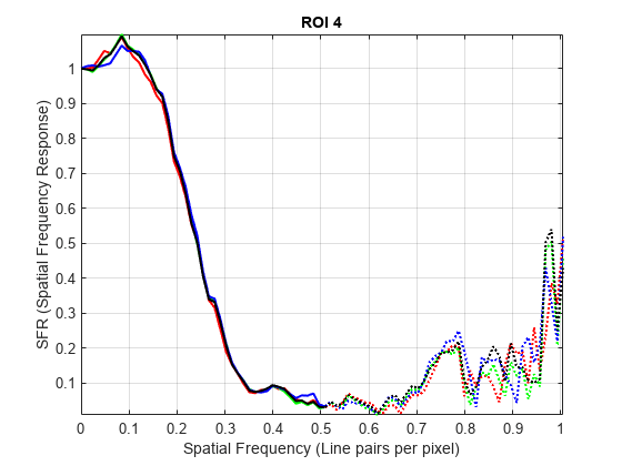
Display the SFR plot for the first four ROIs.
plotSFR(sharpnessTable,ROIIndex=1:4,displayLegend=false,displayTitle=true)

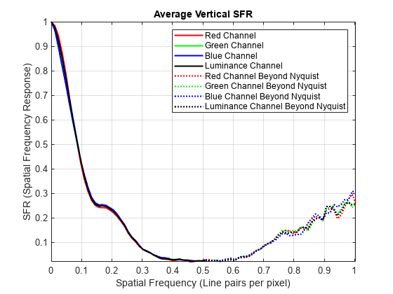
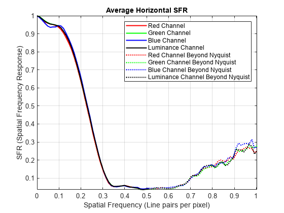
Display the average SFR of the averaged vertical and horizontal edges. The average vertical SFR drops off more rapidly than the average horizontal SFR. Therefore, the average vertical edge is less sharp than the average horizontal edge.
plotSFR(aggregateSharpnessTable)
Measure Chromatic Aberration
Measure chromatic aberration at all slanted edge ROIs.
chTable = measureChromaticAberration(chart);
Plot the normalized intensity profile of the three color channels in the first ROI. Store the normalized edge profile in a separate variable, edgeProfile, for clarity.
roi_index = 1;
edgeProfile = chTable.normalizedEdgeProfile{roi_index};

figure
p = length(edgeProfile.normalizedEdgeProfile_R);
plot(1:p,edgeProfile.normalizedEdgeProfile_R,"r", ...
     1:p,edgeProfile.normalizedEdgeProfile_G,"g", ...
     1:p,edgeProfile.normalizedEdgeProfile_B,"b")
xlabel("Pixel")
ylabel("Normalized Intensity")
title("ROI "+roi_index+" with Aberration "+chTable.aberration(1))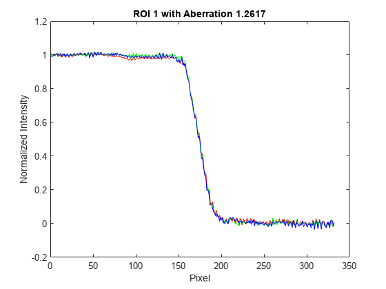
The color channels have similar normalized intensity profiles, and not much color fringing is visible along the edge.
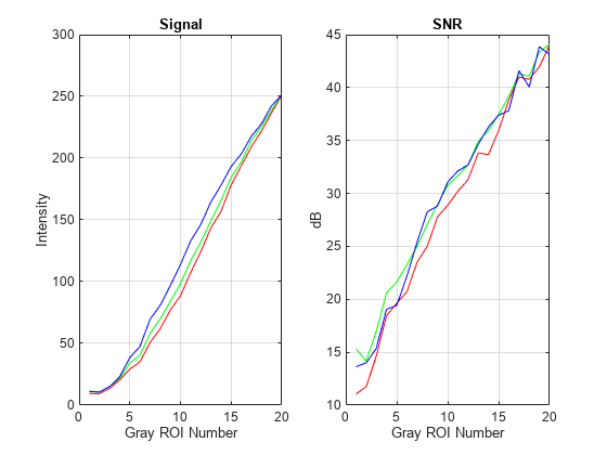
Measure Noise
Measure noise using the 20 gray patch ROIs.
noiseTable = measureNoise(chart);
Plot the average raw signal and the signal-to-noise ratio (SNR) in each grayscale ROI.
figure
subplot(1,2,1)
plot(noiseTable.ROI,noiseTable.MeanIntensity_R,"r", ...
    noiseTable.ROI,noiseTable.MeanIntensity_G,"g", ...
    noiseTable.ROI,noiseTable.MeanIntensity_B,"b")
title("Signal")
ylabel("Intensity")
xlabel("Gray ROI Number")
grid on

subplot(1,2,2)
plot(noiseTable.ROI,noiseTable.SNR_R,"r", ...
    noiseTable.ROI,noiseTable.SNR_G,"g", ...
    noiseTable.ROI,noiseTable.SNR_B,"b")
title("SNR")
ylabel("dB")
xlabel("Gray ROI Number")
grid on
Estimate Illuminant
Estimate the scene illumination using the 20 gray patch ROIs. The illuminant has a stronger blue component a weaker red component, which is consistent with the blue tint of the test chart image.
illum = measureIlluminant(chart)
illum = 1×3

  110.9147  116.0008  123.2339
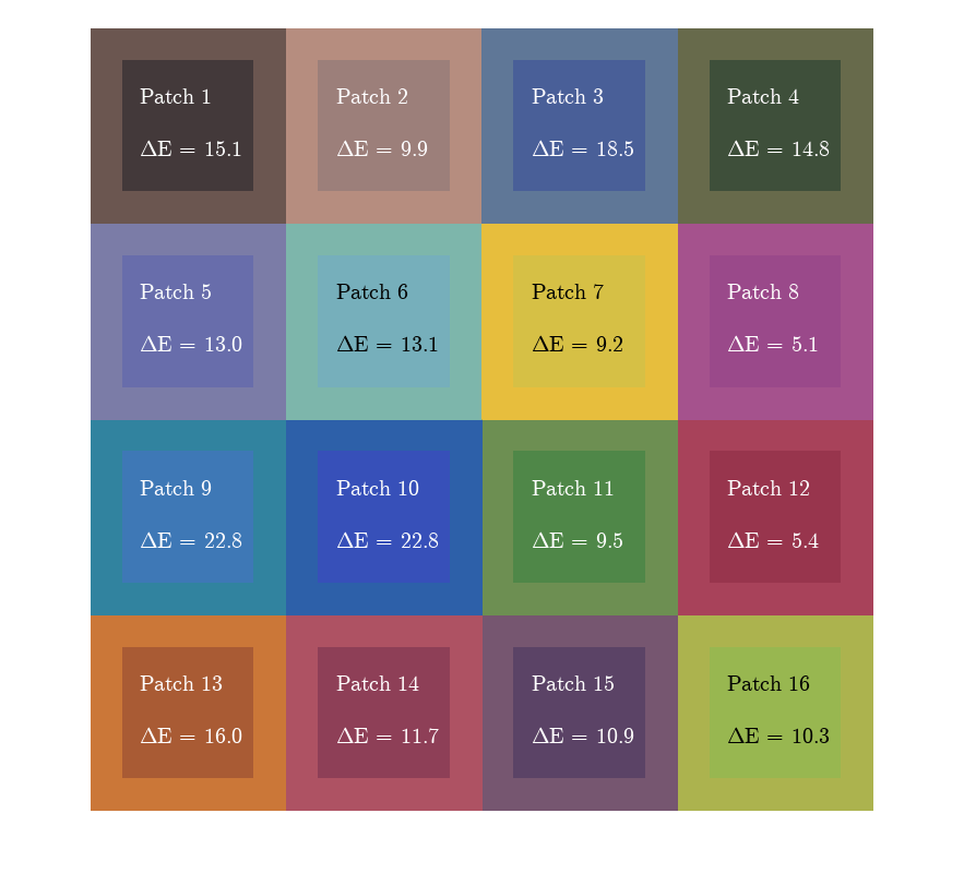
Measure Color Accuracy
Measure color accuracy using the 16 color patch ROIs.
[colorTable,ccm] = measureColor(chart);
Display the average measured color and the expected color of the ROIs. Display the color accuracy measurement, Delta_E. The closer the Delta_E value is to 1, the less perceptible the color difference is. Typical values of Delta_E range from 3 to 6 for printing, and up to 20 in other commercial applications.
figure
displayColorPatch(colorTable)
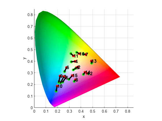
Plot the measured and reference colors in the CIE 1976 L*a*b* color space on a chromaticity diagram. Red circles indicate the reference color. Green circles indicate the measured color of each color patch.
figure
plotChromaticity(colorTable)
You can use the color correction matrix, ccm, to color-correct the test chart images. For an example, see Correct Colors Using Color Correction Matrix.
References
[1] Imatest®. "Esfr". https://www.imatest.com/mathworks/esfr/.
See Also
esfrChart | displayChart | measureSharpness | measureChromaticAberration | measureIlluminant | measureNoise | measureColor