Classify Breast Tumors from Ultrasound Images Using Radiomics Features

This example uses:

This example shows how to use radiomics features to classify breast tumors as benign or malignant from breast ultrasound images.

Radiomics extracts a large number of features from medical images related to the shape, intensity distribution, and texture of the specified region of interest (ROI). The extracted radiomics features contain useful information of the medical image that you can use in a classification application for automated diagnosis. This example extracts radiomics features from the tumor regions of breast ultrasound images and uses these features in a deep learning network to classify whether the tumor is benign or malignant.

About the Data Set

This example uses the Breast Ultrasound Images (BUSI) data set [1]. The BUSI data set contains 2-D ultrasound images stored in the PNG file format. The total size of the data set is 196 MB. The data set contains 133 normal scans that have no tumors, 437 scans with benign tumors, and 210 scans with malignant tumors. Each ultrasound image has a corresponding tumor mask image and a label of normal, benign, or malignant. The tumor mask labels have been reviewed by clinical radiologists [1]. The normal scans do not have any tumor regions in their corresponding tumor mask images. Thus, this example uses images from only the tumor groups.

Download Data Set

Download and unzip the data set.

zipFile = matlab.internal.examples.downloadSupportFile("image","data/Dataset_BUSI.zip");
filepath = fileparts(zipFile);
unzip(zipFile,filepath)

Load and Prepare Data

Prepare the data for training by performing these tasks.

Label each image as normal, benign, or malignant, based on the name of its folder.
Separate the ultrasound and mask images.
Retain images from only the tumor groups.
Create a variable to store labels.

Create a variable imageDir that points to the folder containing the downloaded and unzipped data set. Create an image datastore to read and manage the ultrasound image data. Label each image as normal, benign, or malignant, based on the name of its folder.

imageDir = fullfile(filepath,"Dataset_BUSI_with_GT");
ds = imageDatastore(imageDir,IncludeSubfolders=true,LabelSource="foldernames");

Create a subset of the image datastore containing only the ultrasound images by selecting only files whose names do not contain "mask".

imgds = subset(ds,find(~contains(ds.Files,"mask")));

Create a subset of the image datastore containing only the tumor mask images corresponding to the ultrasound images by selecting all files whose names contain "mask.png".

maskds = subset(ds,find(contains(ds.Files,"mask.png")));

Remove the ultrasound images and the tumor mask images for the images labeled normal, as they do not contain any tumor regions.

imgds = subset(imgds,imgds.Labels~="normal");
maskds = subset(maskds,maskds.Labels~="normal");

Create a vector named labels from the labels of the ultrasound image datastore. The removecats function removes unused categories from a categorical array. Remove the unused category "normal" from labels.

labels = imgds.Labels;
labels = removecats(labels);

View Sample Data

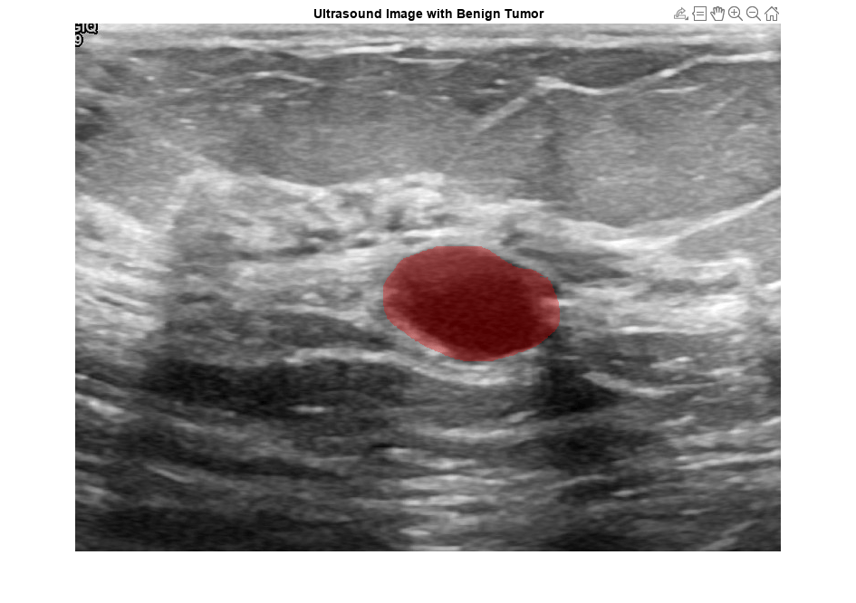
View an ultrasound image that contains a benign tumor with the tumor mask on the image.

benignIdx = find(imgds.Labels == "benign");
benignImage = readimage(imgds,benignIdx(146));
benignMask = readimage(maskds,benignIdx(146));
B = labeloverlay(benignImage,benignMask,Transparency=0.7,Colormap="hsv");
figure
imshow(B)
title("Ultrasound Image with Benign Tumor")

View an ultrasound image that contains a malignant tumor with the tumor mask on the image.

malignantIdx = find(imgds.Labels == "malignant");
malignantImage = readimage(imgds,malignantIdx(200));
malignantMask = readimage(maskds,malignantIdx(200));
B = labeloverlay(malignantImage,malignantMask,Transparency=0.7,Colormap="hsv");
figure
imshow(B)
title("Ultrasound Image with Malignant Tumor")

Create Training and Test Data Sets

Compute the number of ultrasound images in the image datastore.

n = length(imgds.Files)

n = 647

idx = 1:n;

Split the data into 70 percent training data and 30 percent test data using holdout validation.

rng("default")
p = 0.3;
datapartition = cvpartition(n,"Holdout",p);
idxTrain = training(datapartition);
idxTest = test(datapartition);

Create separate vectors for the labels of the training and test data.

labelsTrain = labels(idxTrain);
labelsTest = labels(idxTest);

Compute Radiomics Features for Training Data

The shape of breast tumors in a medical image is very informative for the purpose of classifying breast tumors as benign or malignant. Thus, in this example, you compute the shape-related radiomics features from the tumor regions of the breast ultrasound images.

Create an empty table named radiomicsFeaturesTrain.

radiomicsFeaturesTrain = table;

For each ultrasound image in the training data, read the ultrasound image and the corresponding tumor mask from their respective datastores, pad them to create volumes from the images, and create medicalVolume objects for the ultrasound images and the tumor masks. Create a radiomics object using the ultrasound medical volume as the data and the tumor mask medical volume as the ROI labels. Compute the shape features of the radiomics object, remove the variable LabelID, and append the features to radiomicsFeaturesTrain. The feature computation may take a long time depending on your system configuration.

t = 1;
for i = idx(idxTrain) 
    img = readimage(imgds,i);
    img = im2gray(img);
    img = cat(3,img,zeros([size(img) 2],class(img)));
    volGeometry = medicalref3d(size(img));
    data = medicalVolume(img,volGeometry);
    data.Voxels = squeeze(data.Voxels);

    maskimg = readimage(maskds,i);
    maskimg = im2uint8(maskimg);
    maskimg = cat(3,maskimg,zeros([size(maskimg) 2],class(maskimg)));
    volGeometry = medicalref3d(size(maskimg));
    roiData = medicalVolume(maskimg,volGeometry);
    roiData.Voxels = squeeze(roiData.Voxels);

    R = radiomics(data,roiData);
    S = shapeFeatures(R,SubType="2D");
    S = removevars(S,"LabelID");
    radiomicsFeaturesTrain(t,:) = S;
    t = t + 1;
end

Convert the table radiomicsFeaturesTrain to an array. Save the feature names in the variable featureNames.

radiomicsFeaturesTrain = table2array(radiomicsFeaturesTrain);
featureNames = S.Properties.VariableNames;

Remove Redundant Radiomics Features

Compute the number of features.

f = size(radiomicsFeaturesTrain,2)

f = 23

Calculate the correlation coefficients between each pair of radiomics features in the training data.

featureCorrTrain = corrcoef(radiomicsFeaturesTrain);

If the magnitude of the correlation coefficient between two radiomics features is greater than or equal to 0.95, the features are redundant with one another. Remove each redundant feature from the training and test data, as well as from the list of feature names.

selectedFeatures = true(1,f);
for i = 1:f-1
    if isnan(featureCorrTrain(i,i))
        selectedFeatures(i) = false;
    end
    if selectedFeatures(i)
        for j = i+1:f
            if abs(featureCorrTrain(i,j)) >= 0.95
                selectedFeatures(j) = false;
            end
        end
    end
end
radiomicsFeaturesTrain = radiomicsFeaturesTrain(:,selectedFeatures);
featureNames = featureNames(selectedFeatures);

Visualize Radiomics Features

Compute the number of features after feature selection.

f = size(radiomicsFeaturesTrain,2)

f = 12

Create a logical vector that corresponds to the labels of the training data, representing benign labels with the value false and malignant labels with the value true.

labelsTrainLogical = labelsTrain == "malignant";

Visualize each selected feature for the training data alongside their labels. The first bar in the visualization shows the ground truth classification of the training data, with benign tumors indicated in blue and malignant tumors indicated in yellow. The rest of the bars show each of the selected features. Note that, although the colormap of each feature is different, the trend of each feature changes where the malignancy changes. For example, for the VolumeDensityConvexHull2D feature, the bottom portion of the bar corresponding to malignant tumors is more blue than the upper portion corresponding to benign tumors.

figure(Position=[0 0 1500 500])
tiledlayout(1,f + 1)
nexttile
imagesc(labelsTrainLogical)
xticklabels({})
yticklabels({})
ylabel("Malignancy",Interpreter="none")
for i = 1:f
    nexttile
    imagesc(radiomicsFeaturesTrain(:,i))
    xticklabels({})
    yticklabels({})
    ylabel(featureNames{i},Interpreter="none")
end

Train Deep Learning Network

Use the training data and the corresponding labels to train a deep learning classification neural network using the fitcnet (Statistics and Machine Learning Toolbox) function with sigmoid activation and three fully connected layers, which have 2, 36, and 2 outputs respectively. Standardize each numeric predictor variable, and set the regularization term strength Lambda to 0.00016437.

This example uses the deep learning classification neural network model and hyperparameters determined using the fitcauto (Statistics and Machine Learning Toolbox) function.

model = fitcauto(radiomicsFeaturesTrain,labelsTrain,Learners="net")

model = fitcnet(radiomicsFeaturesTrain,labelsTrain,Activations="sigmoid",Standardize=true,Lambda=0.00016437,LayerSizes=[2 36 2]);

For an example on using fuzzy inference systems for classification of breast tumors, see Classify Breast Tumors from Ultrasound Images Using Fuzzy Inference System (Fuzzy Logic Toolbox).

Compute Radiomics Features for Test Data

Compute the shape features for the test data using a similar process as for the training data. The feature computation may take a long time depending on your system configuration. Remove the same redundant features as from the training data.

radiomicsFeaturesTest = table;
t = 1;
for i = idx(idxTest) 
    img = readimage(imgds,i);
    img = im2gray(img);
    img = cat(3,img,zeros([size(img) 2],class(img)));
    volGeometry = medicalref3d(size(img));
    data = medicalVolume(img,volGeometry);
    data.Voxels = squeeze(data.Voxels);

    maskimg = readimage(maskds,i);
    maskimg = im2uint8(maskimg);
    maskimg = cat(3,maskimg,zeros([size(maskimg) 2],class(maskimg)));
    volGeometry = medicalref3d(size(maskimg));
    roiData = medicalVolume(maskimg,volGeometry);
    roiData.Voxels = squeeze(roiData.Voxels);

    R = radiomics(data,roiData);
    S = shapeFeatures(R,SubType="2D");
    S = removevars(S,"LabelID");
    radiomicsFeaturesTest(t,:) = S;
    t = t + 1;
end
radiomicsFeaturesTest = table2array(radiomicsFeaturesTest);
radiomicsFeaturesTest = radiomicsFeaturesTest(:,selectedFeatures);

Classify Test Data using Trained Deep Learning Network

Use the trained model and the predict (Statistics and Machine Learning Toolbox) function to predict whether each test data image contains a benign or malignant tumor. False negatives can be more undesirable than false positives in automated medical diagnosis. Adjust the misclassification cost of the model to assign higher cost to false negatives than false positives during prediction.

falseNegativeCost = 8;
model.Cost = [0 1;falseNegativeCost 0];
predictedLabelsTest = predict(model,radiomicsFeaturesTest);

Evaluate Classification Accuracy

Compute the accuracy of the predicted labels from the confusion matrix.

confusionMatrix = confusionmat(labelsTest,predictedLabelsTest)

confusionMatrix = 2×2

   125     3
     1    65

accuracy = sum(diag(confusionMatrix))/sum(confusionMatrix,"all")

accuracy = 0.9794

Create a normalized confusion matrix chart from the true labels labelsTest and the predicted labels predictedLabelsTest.

figure
confusionchart(labelsTest,predictedLabelsTest,Normalization="total-normalized")

References

[1] Al-Dhabyani, Walid, Mohammed Gomaa, Hussien Khaled, and Aly Fahmy. “Dataset of Breast Ultrasound Images.” Data in Brief 28 (February 2020): 104863. https://doi.org/10.1016/j.dib.2019.104863.