Minimice el rango de búsqueda en la coincidencia de escaneo Lidar basada en cuadrícula usando IMU
Este ejemplo muestra cómo utilizar una unidad de medición inercial (IMU) para minimizar el rango de búsqueda del ángulo de rotación para algoritmos de coincidencia de escaneo. Las lecturas del sensor IMU se utilizan para estimar la orientación del vehículo y se especifican como la estimación inicial para la función matchScansGrid. Este método de estimación de pose inicial se compara con el algoritmo base que supone una estimación inicial de [0 0 0].
Cargar datos registrados
Cargue el archivo MAT, loggedLidarAndIMUData.mat. Este archivo contiene escaneos LiDAR , lecturas del acelerómetro y lecturas de giroscopios, y las marcas de tiempo correspondientes.
rng(1); % Fixed RNG seed for repeatibility
load('loggedLidarAndIMUData', ...
    'tLidar', 'lidarScans', ...
    'imuFs', 'tIMU', 'accel', 'gyro');

startIdx = 1;
endIdx = numel(lidarScans)-1;
Sincronizar índices de tiempo IMU con índices de tiempo Lidar
La IMU y el lidar se actualizan a diferentes velocidades de muestreo. Cree un arreglo que asigne lidar a índices IMU.
lidarToIMUIndices = zeros(size(tLidar));
for i = 1:numel(tLidar)
    [~, lidarToIMUIndices(i)] = min(abs(tLidar(i) - tIMU));
end
Estimar la guiñada a partir de IMU
Estime la orientación a partir de las lecturas del acelerómetro y del giroscopio como un cuaternión utilizando el objeto imufilter. Luego, calcule las guiñadas relativas entre escaneos LIDAR sucesivos convirtiendo los cuaterniones en ángulos de Euler.
orientFilt = imufilter('SampleRate', imuFs);
q = orientFilt(accel, gyro);

% Calculate relative yaws
eulerAngs = euler(q(lidarToIMUIndices(1+(startIdx:endIdx))) ...
    .* conj(q(lidarToIMUIndices(startIdx:endIdx))), 'ZYX', 'frame');
imuYaws = eulerAngs(:,1);
Ejecute la coincidencia de análisis y registre los resultados
Ejecute la función matchScansGrid con dos opciones diferentes:
Suposición inicial predeterminada y rango de búsqueda
Suposición inicial basada en lecturas del sensor IMU con un rango de búsqueda pequeño
Iterar a través de todas las lecturas de escaneos LiDAR , ejecutando matchScansGrid con cada par de escaneos secuenciales. Registre los tiempos de procesamiento para cada llamada de función y las salidas de pose relativas de la coincidencia de escaneo. Para visualizar los escaneos transformados en función de la solución, configure plotSolutions en 1. Sin embargo, en este ejemplo, la diferencia de pose entre las dos opciones diferentes no se nota.
smallSearchRange = pi/8;
plotSolutions = 0;

% Initialize time values and relative pose arrays
timeDefaultSearch = NaN(endIdx - startIdx + 1,1);
timeSmallSearchWithIMU = NaN(endIdx - startIdx + 1,1);
allRelPosesDefault = NaN(endIdx - startIdx + 1,3);
allRelPosesIMU = NaN(endIdx - startIdx + 1,3);

for idx = startIdx:endIdx
    scan1 = lidarScans(idx);
    scan2 = lidarScans(idx+1);

    yaw = imuYaws(idx);
    initGuess = [0 0 yaw];

    % Run scan matching with default values.
    tic;
    relPose = matchScansGrid(scan2, scan1);
    timeDefaultSearch(idx) = toc;

    allRelPosesDefault(idx,:) = relPose;

    % Run scan matching with IMU-based initial yaw and small search range.
    tic;
    relPose = matchScansGrid(scan2, scan1, 'InitialPose', initGuess, ...
        'RotationSearchRange', smallSearchRange);
    timeSmallSearchWithIMU(idx) = toc;
    allRelPosesIMU(idx,:) = relPose;

    % Set plot solutions to 1 to turn on scan visualization.
    if plotSolutions == 1
        figure(cfg,'Visibile','on')
        plot(scan1)
        hold on
        plot(transformScan(scan2, allRelPosesDefault(idx,:)))
        plot(transformScan(scan2, allRelPosesIMU(idx,:)))
        hold off
        legend('Ref Scan','Default', ...
            'Small Search Range + IMU',...
            'Location','northwest')
        title(sprintf('Matched Lidar Scans %d and %d', i, i+1))
    end

end
Comparar resultados
Visualice y compare los resultados de coincidencia del escaneo. Muestre el tiempo total de procesamiento como un gráfico de barras. Luego, compare el tiempo de cada iteración.
figure
title('Scan Matching Processing Time')
bar(categorical({'Default','IMU + Small Search'}), ...
    [sum(timeDefaultSearch),sum(timeSmallSearchWithIMU)])
ylabel('time (s)')
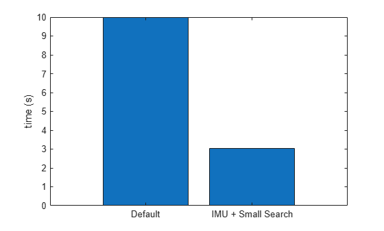
figure
title('Difference in Interation Time')
plot(startIdx:endIdx,(timeDefaultSearch - timeSmallSearchWithIMU))
ylabel('Time (seconds)')
xlabel('Iteration')
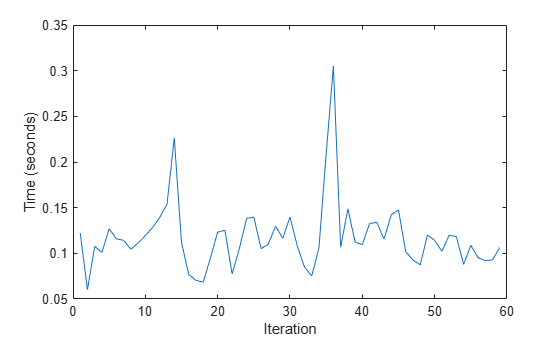
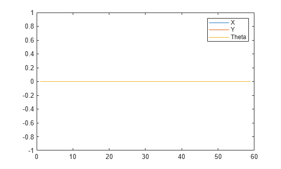
Según los resultados del tiempo, especificar las lecturas del sensor IMU como una estimación para el algoritmo de coincidencia de escaneo mejora el tiempo de cada iteración. Como paso final, puede verificar que la diferencia en la pose estimada no sea significativa. Para este ejemplo, todas las poses de matchScansGrid son iguales.
figure
title('Difference in Pose Values')
plot(allRelPosesDefault-allRelPosesIMU)
legend('X','Y','Theta')