Illustrating Three Approaches to GPU Computing: The Mandelbrot Set

Setup

The values below specify a highly zoomed part of the Mandelbrot Set in the valley between the main cardioid and the p/q bulb to its left.

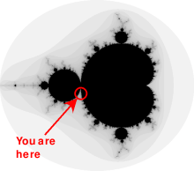
A 1000x1000 grid of real parts (X) and imaginary parts (Y) is created between these limits and the Mandelbrot algorithm is iterated 500 times at each grid location.

maxIterations = 500;
gridSize = 1000;
xlim = [-0.748766713922161, -0.748766707771757];
ylim = [ 0.123640844894862,  0.123640851045266];

The Mandelbrot Set in MATLAB

Below is an implementation of the Mandelbrot Set using standard MATLAB commands running on the CPU. This is based on the code provided in Cleve Moler's Experiments with MATLAB e-book. Time the execution on the CPU using tic and toc.

Setup the two-dimensional grid of complex values.

tic;
x = linspace(xlim(1),xlim(2),gridSize);
y = linspace(ylim(1),ylim(2),gridSize);

[xGrid,yGrid] = meshgrid(x,y);
z0 = xGrid + 1i*yGrid;

For 500 iterations, calculate the next value of a point on the complex grid z by squaring the previous value and adding its initial value, z0. Count the number of iterations for which the magnitude of z is less than or equal to two. This calculation is vectorized such that every location is updated at once.

cpuCount = ones(size(z0));
z = z0;
for n = 0:maxIterations
    z = z.*z + z0;
    inside = abs(z)<=2;
    cpuCount = cpuCount + inside;
end
cpuCount = log(cpuCount);
cpuTime = toc

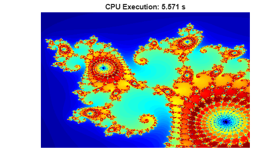
cpuTime = 4.4007

Plot the natural logarithm of the count.

figure
imagesc(x,y,cpuCount);
c = colormap([jet;flipud(jet);0 0 0]);
axis off
title(sprintf("CPU Execution: %1.3f s",cpuTime));

Using gpuArray

When MATLAB encounters data on the GPU, calculations with that data are performed on the GPU. The class gpuArray provides GPU versions of many functions that you can use to create data arrays, including the linspace, logspace, and meshgrid functions needed here. Similarly, the count array is initialized directly on the GPU using the function ones.

Ensure that your desired GPU is available and selected.

gpu = gpuDevice;
disp(gpu.Name + " GPU selected.")

NVIDIA RTX A5000 GPU selected.

Call the naiveGPUMandelbrot function. The supporting function naiveGPUMandelbrot applies the Mandelbrot algorithm for each point on the grid on the GPU and is provided at the end of this examples.

[x,y,naiveGPUCount] = naiveGPUMandelbrot(xlim,ylim,gridSize,maxIterations);

Time the execution of the function on the GPU using gputimeit. For functions that use the GPU, gputimeit is better than tic and toc or timeit because it ensures that all operations on the GPU finish before recording the elapsed time.

naiveGPUTime = gputimeit(@() naiveGPUMandelbrot(xlim,ylim,gridSize,maxIterations))

naiveGPUTime = 0.2181

Element-wise Operation

Noting that the algorithm is operating equally on every element of the input, we can place the code in a function and call it using arrayfun. The function processMandelbrotElement is provided as a supporting function at the end of this example. For gpuArray inputs, the function used with arrayfun gets compiled into native GPU code.

An early abort has been introduced into the function processMandelbrotElement because this function processes only a single element. For most views of the Mandelbrot Set a significant number of elements stop very early and this can save a lot of processing. The for-loop has also been replaced by a while-loop because they are usually more efficient. This function makes no mention of the GPU and uses no GPU-specific features.

Using arrayfun causes MATLAB to make one call to a parallelized GPU operation that performs the whole calculation, instead of many thousands of calls to separate GPU-optimized operations (at least 6 per iteration). The first time you call arrayfun to run a particular function on the GPU, there is some overhead time to set up the function for GPU execution. Subsequent calls of arrayfun with the same function can run faster.

Setup the two-dimensional grid of complex values.

xGrid = gpuArray(xGrid);
yGrid = gpuArray(yGrid);

Using arrayfun, apply the Mandelbrot algorithm for each point on the grid.

gpuArrayfunCount = arrayfun(@processMandelbrotElement, ...
                  xGrid,yGrid,maxIterations);

Time the arrayfun execution using gputimeit.

gpuArrayfunTime = gputimeit(@() arrayfun(@processMandelbrotElement, ...
                  xGrid,yGrid,maxIterations))

gpuArrayfunTime = 0.0308

Working with CUDA

In Experiments in MATLAB performance is improved by converting the basic algorithm to a C-Mex function. If you are willing to do some work in C/C++, then you can use Parallel Computing Toolbox to call pre-written CUDA kernels using MATLAB data. For more details on using CUDA kernels in MATLAB, see Run CUDA or PTX Code on GPU.

A CUDA/C++ implementation of the element processing algorithm is provided with this example, pctdemo_processMandelbrotElement.cu. The part of the CUDA/C++ code that executes the Mandelbrot algorithm for a single location is given below.

__device__
unsigned int doIterations( double const realPart0, 
                           double const imagPart0, 
                           unsigned int const maxIters ) {
   // Initialize: z = z0
   double realPart = realPart0;
   double imagPart = imagPart0;
   unsigned int count = 0;
   // Loop until escape
   while ( ( count <= maxIters )
          && ((realPart*realPart + imagPart*imagPart) <= 4.0) ) {
      ++count;
      // Update: z = z*z + z0;
      double const oldRealPart = realPart;
      realPart = realPart*realPart - imagPart*imagPart + realPart0;
      imagPart = 2.0*oldRealPart*imagPart + imagPart0;
   }
   return count;
}

Compile this file into a parallel thread execution (PTX) file using mexcuda.

mexcuda -ptx pctdemo_processMandelbrotElement.cu

Building with 'NVIDIA CUDA Compiler'.
MEX completed successfully.

Create a parallel.gpu.CUDAKernel object by passing the CUDA file and the PTX file to the parallel.gpu.CUDAKernel function.

cudaFilename = "pctdemo_processMandelbrotElement.cu";
ptxFilename = "pctdemo_processMandelbrotElement.ptx";
kernel = parallel.gpu.CUDAKernel(ptxFilename,cudaFilename);

One GPU thread is required per location in the Mandelbrot Set, with the threads grouped into blocks. The kernel indicates how big a thread-block is. Calculate the number of thread-blocks required, and set the GridSize property of the kernel (effectively the number of thread blocks that will be launched independently by the GPU) accordingly.

numElements = numel(xGrid);
kernel.ThreadBlockSize = [kernel.MaxThreadsPerBlock,1,1];
kernel.GridSize = [ceil(numElements/kernel.MaxThreadsPerBlock),1];

Evaluate the kernel using feval.

count = zeros(size(xGrid),"gpuArray");
gpuCUDAKernelCount = feval(kernel,count,xGrid,yGrid,maxIterations,numElements);

Time the kernel execution using gputimeit.

gpuCUDAKernelTime = gputimeit(@() feval(kernel,count,xGrid,yGrid,maxIterations,numElements));

Summary

Plot the results from the different methods and compare the execution times.

method = ["Naive GPU Execution" "GPU Execution Using arrayfun" "CUDAKernel Execution"];
count = cat(3,naiveGPUCount,gpuArrayfunCount,gpuCUDAKernelCount);
time = [naiveGPUTime gpuArrayfunTime gpuCUDAKernelTime];

figure
colormap(c)
tiledlayout("flow")
nexttile
imagesc(x,y,cpuCount);
axis off
title(sprintf("CPU Execution: %1.3f s",cpuTime));

for idx = 1:3
nexttile
imagesc(x,y,count(:,:,idx))
axis off
title(sprintf("%s: %1.3f s \n  (%1.1fx faster)", ...
    method(idx),time(idx),cpuTime/time(idx)))
end

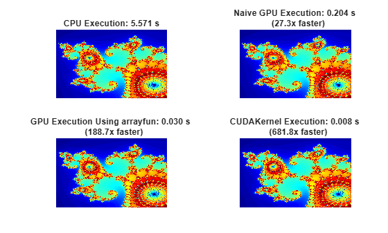
This example has shown three ways in which a MATLAB algorithm can be adapted to make use of GPU hardware:

The code in this example was timed on a Windows® 10, Intel® Xeon® W-2133 @ 3.60 GHz test system with an NVIDIA® RTX A5000 GPU.

Supporting Functions

The supporting function naiveGPUMandelbrot creates a two-dimensional grid of complex values and counts the number of iterations before the complex value number (x0,y0) jumps outside a circle of radius 2 on the complex plane. Each iteration involves mapping z = z^2 + z0 where z0 = x0 + i*y0. The function returns the grid coordinate vectors and the log of the iteration count at escape or maxIterations if the point did not escape. By initializing data on the GPU and operating on this data, the naiveGPUMandelbrot function executes the Mandelbrot algorithm on the GPU.

function [x,y,count] = naiveGPUMandelbrot(xlim,ylim,gridSize,maxIterations)

x = gpuArray.linspace(xlim(1),xlim(2),gridSize);
y = gpuArray.linspace(ylim(1),ylim(2),gridSize);
[xGrid,yGrid] = meshgrid(x,y);

z0 = complex(xGrid,yGrid);
count = ones(size(z0),"gpuArray");
z = z0;

for n = 0:maxIterations
    z = z.*z + z0;
    inside = abs(z)<=2;
    count = count + inside;
end

count = log(count);

end

The supporting function processMandelbrotElement creates a two-dimensional grid of complex values and counts the number of iterations before the complex value number (x0,y0) jumps outside a circle of radius 2 on the complex plane. Each iteration involves mapping z = z^2 + z0 where z0 = x0 + i*y0. The function returns the log of the iteration count at escape or maxIterations if the point did not escape.

function count = processMandelbrotElement(x0,y0,maxIterations)

z0 = complex(x0,y0);
z = z0;
count = 1;

while (count <= maxIterations) && (abs(z) <= 2)
    count = count + 1;
    z = z*z + z0;
end

count = log(count);

end