interpolateStrain
Interpolate strain at arbitrary spatial locations
Syntax
Description
intrpStrain = interpolateStrain(structuralresults,xq,yq)xq and yq. For transient and
frequency-response structural problems, interpolateStrain
interpolates strain for all time or frequency steps, respectively.
intrpStrain = interpolateStrain(structuralresults,xq,yq,zq)xq, yq, and
zq.
intrpStrain = interpolateStrain(structuralresults,querypoints)querypoints.
Examples
Create an femodel object for static structural analysis and include a unit square geometry into the model.
model = femodel(AnalysisType="structuralStatic", ...
                Geometry=@squareg);
Plot the geometry.
pdegplot(model.Geometry,EdgeLabels="on")
xlim([-1.1 1.1])
ylim([-1.1 1.1])
Switch the problem type to plane-strain.
model.PlanarType = "planeStrain";Specify Young's modulus and Poisson's ratio.
model.MaterialProperties = ...
    materialProperties(YoungsModulus=210E3, ...
                       PoissonsRatio=0.3);
Specify the x-component of the enforced displacement for edge 1.
model.EdgeBC(1) = edgeBC(XDisplacement=0.001);
Specify that edge 3 is a fixed boundary.
model.EdgeBC(3) = edgeBC(Constraint="fixed");Generate a mesh and solve the problem.
model = generateMesh(model);
R = solve(model);
Create a grid and interpolate the x- and y-components of the normal strain to the grid.
v = linspace(-1,1,101);
[X,Y] = meshgrid(v);
intrpStrain = interpolateStrain(R,X,Y);
Reshape the x-component of the normal strain to the shape of the grid and plot it.
exx = reshape(intrpStrain.exx,size(X));
px = pcolor(X,Y,exx);
px.EdgeColor="none";
colorbar
axis equal

Reshape the y-component of the normal strain to the shape of the grid and plot it.
eyy = reshape(intrpStrain.eyy,size(Y));
figure
py = pcolor(X,Y,eyy);
py.EdgeColor="none";
colorbar
axis equal

Analyze a bimetallic cable under tension, and interpolate strain on a cross-section of the cable.
Create and plot a geometry representing a bimetallic cable.
gm = multicylinder([0.01,0.015],0.05);
pdegplot(gm,FaceLabels="on", ...
            CellLabels="on", ...
            FaceAlpha=0.5)

Create an femodel for static structural analysis and include the geometry into the model.
model = femodel(AnalysisType="structuralStatic", ...
                Geometry=gm);
Specify Young's modulus and Poisson's ratio for each metal.
model.MaterialProperties(1) = ...
    materialProperties(YoungsModulus=110E9, ...
                       PoissonsRatio=0.28);
model.MaterialProperties(2) = ...
    materialProperties(YoungsModulus=210E9, ...
                       PoissonsRatio=0.3);
Specify that faces 1 and 4 are fixed boundaries.
model.FaceBC([1 4]) = faceBC(Constraint="fixed");Specify the surface traction for faces 2 and 5.
model.FaceLoad([2 5]) = faceLoad(SurfaceTraction=[0;0;100]);
Generate a mesh and solve the problem.
model = generateMesh(model);
R = solve(model)
R =
  StaticStructuralResults with properties:

      Displacement: [1×1 FEStruct]
            Strain: [1×1 FEStruct]
            Stress: [1×1 FEStruct]
    VonMisesStress: [23098×1 double]
              Mesh: [1×1 FEMesh]
Define the coordinates of a midspan cross-section of the cable.
[X,Y] = meshgrid(linspace(-0.015,0.015,50));
Z = ones(size(X))*0.025;
Interpolate the strain and plot the result.
intrpStrain = interpolateStrain(R,X,Y,Z);
surf(X,Y,reshape(intrpStrain.ezz,size(X)))

Alternatively, you can specify the grid by using a matrix of query points.
querypoints = [X(:),Y(:),Z(:)]';
intrpStrain = interpolateStrain(R,querypoints);
surf(X,Y,reshape(intrpStrain.ezz,size(X)))

Interpolate the strain at the geometric center of a beam under a harmonic excitation.
Create and plot a beam geometry.
gm = multicuboid(0.06,0.005,0.01);
pdegplot(gm,FaceLabels="on",FaceAlpha=0.5)
view(50,20)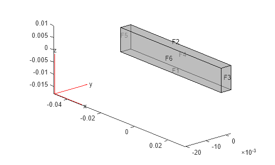
Create an femodel object for transient structural analysis and include the geometry into the model.
model = femodel(AnalysisType="structuralTransient", ...
                Geometry=gm);
Specify Young's modulus, Poisson's ratio, and the mass density of the material.
model.MaterialProperties = ...
    materialProperties(YoungsModulus=210E9, ...
                       PoissonsRatio=0.3, ...
                       MassDensity=7800);
Fix one end of the beam.
model.FaceBC(5) = faceBC(Constraint="fixed");Apply a sinusoidal displacement along the y-direction on the end opposite the fixed end of the beam.
yDisplacementFunc = ...
@(location,state) ones(size(location.y))*1E-4*sin(50*state.time);
model.FaceBC(3) = faceBC(YDisplacement=yDisplacementFunc);
Generate a mesh.
model = generateMesh(model,Hmax=0.01);
Specify the zero initial displacement and velocity.
model.CellIC = cellIC(Displacement=[0;0;0],Velocity=[0;0;0]);
Solve the problem.
tlist = 0:0.002:0.2;
R = solve(model,tlist);
Interpolate the strain at the geometric center of the beam.
coordsMidSpan = [0;0;0.005];
intrpStrain = interpolateStrain(R,coordsMidSpan);
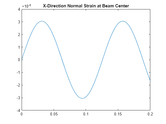
Plot the normal strain at the geometric center of the beam.
plot(R.SolutionTimes,intrpStrain.exx)
title("X-Direction Normal Strain at Beam Center")