EHfields

Electric and magnetic fields of PCB components

Since R2025a

Syntax

[e,h] = EHfields(object,frequency)

EHfields(object,frequency)

[e,h] = EHfields(object,frequency,points)

EHfields(___,Name=Value)

Description

[e,h] = EHfields(object,frequency) calculates the x, y, and z components of the electric and magnetic fields of a rf pcb object at a specified frequency. The fields are calculated at points on the surface of a sphere whose radius is twice that of the radius of a sphere completely enclosing the rf pcb structure.

EHfields(object,frequency) plots the absolute values of the electric and magnetic field vectors along with corresponding signed complex angles at the specified frequency. The multiplication factor with absolute field value is +1 for positive and -1 for negative complex angle. The fields are calculated at points on the surface of a sphere whose radius is twice that of the radius of a sphere completely enclosing the rf pcb structure.

[e,h] = EHfields(object,frequency,points) calculates the x, y, and z components of electric field and magnetic field of a rf pcb object. These fields are calculated at specified points in the space and at a specified frequency. Specify the points in the Cartesian coordinate system.

EHfields(___,Name=Value) plots the electric and magnetic field vectors using one or more name-value arguments (Antenna Toolbox) in addition to any of the input argument combinations in previous syntaxes. For example, ViewField="E" displays only the electric field.

Examples

Plot Electric and Magnetic Fields of Combline Filter

Plot the electric and magnetic fields of a default combline filter at 70 MHz

EHfields(filterCombline,70e6)

Section 2 Title

Description of second code block

a=2;

Calculate Electric and Magnetic Fields of Combline Filter

Calculate the electric and magnetic fields of a combline filter at 70 MHz

h = filterCombline;
[e,h] = EHfields(h,70e6)

e = 3×76 complex
103 ×

  -0.0002 + 0.0000i  -0.0322 - 0.0000i  -0.0024 - 0.0000i   0.0119 + 0.0000i  -0.0075 - 0.0000i  -0.0405 - 0.0000i  -0.0090 - 0.0000i   0.0082 + 0.0000i  -0.0079 - 0.0000i  -0.0247 - 0.0000i   0.0183 + 0.0000i   0.0502 + 0.0000i   0.0220 + 0.0000i  -0.0100 - 0.0000i  -0.0235 - 0.0000i  -0.0437 - 0.0000i  -0.0605 - 0.0000i   0.0132 + 0.0000i   0.0096 - 0.0000i  -0.0159 - 0.0000i  -0.0787 - 0.0000i  -0.0814 - 0.0000i  -0.0123 - 0.0000i   0.0601 + 0.0000i   0.0735 + 0.0000i   0.0561 + 0.0000i  -0.0150 - 0.0000i  -0.0238 - 0.0000i   0.0297 + 0.0000i   0.0641 + 0.0000i   0.0293 + 0.0000i  -0.0043 - 0.0000i  -0.0158 - 0.0000i  -0.0429 - 0.0000i  -0.0628 - 0.0000i  -0.0816 - 0.0000i  -0.0872 - 0.0000i  -0.0012 + 0.0000i   0.0703 + 0.0000i   0.0672 + 0.0000i   0.0394 + 0.0000i   0.0066 + 0.0000i   0.0012 + 0.0000i  -0.0137 - 0.0000i   0.2223 + 0.0001i   0.3214 + 0.0002i  -0.2963 - 0.0001i   0.1566 + 0.0000i   0.1940 + 0.0001i  -0.1030 - 0.0000i
  -0.0034 - 0.0000i   0.0118 + 0.0000i   0.0037 + 0.0000i   0.0056 + 0.0000i  -0.0170 - 0.0000i   0.0149 + 0.0000i   0.0109 + 0.0000i   0.0032 + 0.0000i   0.0180 + 0.0000i   0.0572 + 0.0000i   0.0683 + 0.0000i   0.0252 + 0.0000i  -0.0139 - 0.0000i  -0.0229 - 0.0000i  -0.0193 - 0.0000i  -0.0167 - 0.0000i  -0.0026 - 0.0000i   0.0001 - 0.0000i  -0.0031 - 0.0000i   0.0072 + 0.0000i   0.0535 + 0.0000i   0.1336 + 0.0001i   0.1904 + 0.0001i   0.1648 + 0.0001i   0.0775 + 0.0000i   0.0330 + 0.0000i   0.0249 + 0.0000i   0.0634 + 0.0000i   0.0669 + 0.0000i   0.0039 - 0.0000i  -0.0281 - 0.0000i  -0.0251 - 0.0000i  -0.0222 - 0.0000i  -0.0258 - 0.0000i  -0.0038 - 0.0000i   0.0550 + 0.0000i   0.1535 + 0.0001i   0.2081 + 0.0001i   0.1559 + 0.0001i   0.0574 + 0.0000i   0.0189 + 0.0000i  -0.0012 + 0.0000i  -0.0023 - 0.0000i   0.0091 + 0.0000i   0.2549 + 0.0001i   0.4002 + 0.0002i   0.8740 + 0.0004i   0.2868 + 0.0000i   0.0132 - 0.0001i   0.0713 - 0.0000i
  -0.0314 + 0.0004i  -0.0389 + 0.0004i  -0.0257 + 0.0004i  -0.0283 + 0.0004i  -0.0304 + 0.0004i  -0.0247 + 0.0004i  -0.0287 + 0.0004i  -0.0246 + 0.0004i  -0.0277 + 0.0004i  -0.0145 + 0.0004i  -0.0140 + 0.0004i  -0.0356 + 0.0004i  -0.0477 + 0.0004i  -0.0429 + 0.0004i  -0.0406 + 0.0004i  -0.0463 + 0.0004i  -0.0499 + 0.0004i  -0.0300 + 0.0004i  -0.0296 + 0.0004i  -0.0245 + 0.0004i  -0.0695 + 0.0004i  -0.1221 + 0.0004i  -0.1476 + 0.0004i  -0.1193 + 0.0004i  -0.0686 + 0.0004i  -0.0468 + 0.0004i  -0.0385 + 0.0004i  -0.0651 + 0.0004i  -0.0861 + 0.0004i  -0.0773 + 0.0004i  -0.0538 + 0.0004i  -0.0378 + 0.0004i  -0.0325 + 0.0004i  -0.0291 + 0.0004i  -0.0249 + 0.0004i  -0.0165 + 0.0004i   0.0081 + 0.0004i   0.0312 + 0.0004i   0.0256 + 0.0004i  -0.0038 + 0.0004i  -0.0192 + 0.0004i  -0.0264 + 0.0004i  -0.0287 + 0.0004i  -0.0321 + 0.0004i  -0.4584 + 0.0002i  -1.0351 - 0.0000i  -1.0794 - 0.0001i   0.3612 + 0.0005i   0.3743 + 0.0005i   0.1921 + 0.0004i

h = 3×76 complex
103 ×

   0.0000 - 0.0027i  -0.0000 + 0.0044i   0.0000 - 0.0030i  -0.0000 + 0.0021i   0.0000 - 0.0028i  -0.0000 + 0.0045i   0.0000 - 0.0024i  -0.0000 + 0.0028i   0.0000 - 0.0057i   0.0000 - 0.0100i   0.0000 - 0.0130i   0.0000 - 0.0117i   0.0000 - 0.0084i   0.0000 - 0.0048i   0.0000 - 0.0013i  -0.0000 + 0.0013i  -0.0000 + 0.0039i  -0.0000 + 0.0010i   0.0000 - 0.0011i   0.0000 - 0.0026i  -0.0000 + 0.0087i  -0.0000 + 0.0163i  -0.0000 + 0.0189i  -0.0000 + 0.0126i  -0.0000 + 0.0073i  -0.0000 + 0.0039i   0.0000 - 0.0044i   0.0000 - 0.0088i   0.0000 - 0.0147i   0.0000 - 0.0207i   0.0000 - 0.0151i   0.0000 - 0.0061i  -0.0000 + 0.0003i  -0.0000 + 0.0047i  -0.0000 + 0.0051i  -0.0000 + 0.0082i  -0.0000 + 0.0137i  -0.0000 + 0.0168i  -0.0000 + 0.0147i  -0.0000 + 0.0098i  -0.0000 + 0.0051i  -0.0000 + 0.0022i  -0.0000 + 0.0007i   0.0000 - 0.0012i  -0.0000 + 0.0118i  -0.0001 + 0.0982i   0.0001 - 0.1479i   0.0001 - 0.2531i   0.0001 - 0.1845i   0.0000 - 0.0062i
  -0.0000 + 0.0065i  -0.0000 + 0.0061i   0.0000 - 0.0041i   0.0000 - 0.0048i  -0.0000 + 0.0081i  -0.0000 + 0.0068i   0.0000 - 0.0049i   0.0000 - 0.0048i   0.0000 - 0.0054i   0.0000 - 0.0045i  -0.0000 + 0.0005i  -0.0000 + 0.0058i  -0.0000 + 0.0097i  -0.0000 + 0.0090i  -0.0000 + 0.0099i  -0.0000 + 0.0118i  -0.0000 + 0.0099i   0.0000 - 0.0068i   0.0000 - 0.0075i   0.0000 - 0.0064i  -0.0000 + 0.0088i  -0.0000 + 0.0081i   0.0000 - 0.0011i   0.0000 - 0.0069i   0.0000 - 0.0083i   0.0000 - 0.0066i   0.0000 - 0.0065i   0.0000 - 0.0075i   0.0000 - 0.0040i  -0.0000 + 0.0057i  -0.0000 + 0.0162i  -0.0000 + 0.0133i  -0.0000 + 0.0134i  -0.0000 + 0.0147i  -0.0000 + 0.0109i  -0.0000 + 0.0085i  -0.0000 + 0.0081i  -0.0000 + 0.0008i   0.0000 - 0.0057i   0.0000 - 0.0087i   0.0000 - 0.0073i   0.0000 - 0.0073i   0.0000 - 0.0087i   0.0000 - 0.0071i   0.0000 - 0.0191i   0.0001 - 0.1003i   0.0001 - 0.1002i  -0.0002 + 0.2979i   0.0000 - 0.0159i   0.0000 - 0.0058i
  -0.0000 + 0.0020i   0.0000 - 0.0011i   0.0000 - 0.0012i   0.0000 - 0.0004i   0.0000 - 0.0006i   0.0000 - 0.0007i   0.0000 - 0.0008i   0.0000 - 0.0010i   0.0000 - 0.0010i  -0.0000 + 0.0001i  -0.0000 + 0.0029i  -0.0000 + 0.0090i  -0.0000 + 0.0077i  -0.0000 + 0.0049i  -0.0000 + 0.0042i  -0.0000 + 0.0033i   0.0000 - 0.0006i   0.0000 - 0.0007i   0.0000 - 0.0018i   0.0000 - 0.0020i   0.0000 - 0.0008i   0.0000 - 0.0008i  -0.0000 + 0.0038i  -0.0000 + 0.0039i  -0.0000 + 0.0013i  -0.0000 + 0.0010i   0.0000 - 0.0001i  -0.0000 + 0.0009i  -0.0000 + 0.0001i   0.0000 - 0.0012i   0.0000 - 0.0060i   0.0000 - 0.0024i   0.0000 - 0.0014i   0.0000 - 0.0019i   0.0000 - 0.0015i  -0.0000 + 0.0005i  -0.0000 + 0.0016i  -0.0000 + 0.0038i  -0.0000 + 0.0008i   0.0000 - 0.0026i   0.0000 - 0.0010i   0.0000 - 0.0016i   0.0000 - 0.0017i   0.0000 - 0.0012i  -0.0000 + 0.0080i  -0.0000 + 0.0020i   0.0000 - 0.0917i   0.0001 - 0.2673i   0.0001 - 0.2048i  -0.0000 + 0.0138i

Plot Electric and Magnetic Fields on X-Y Plane

Plot electric and magnetic fields of a corporate power divider in the X-Y plane at 1 MHz

Create the Power Divider Structure

Create the power divider, and specify the size of the ground plane in the X-Y plane. Specify the height along the Z-axis. Set up the 3-D grid coordinates. Set up the cartesian coordinates in space, where p is the number pf points to calculate the E-H field.

h = powerDividerCorporate;
x1 = h.GroundPlaneLength*1.5*0.5;
y1 = h.GroundPlaneWidth*1.5*0.5;
z1 = h.Height*1.5*0.5;
[X,Y,Z] = meshgrid(-x1:0.001:x1,-y1:0.001:y1,-z1:0.005:z1);
p = [X(:)';Y(:)';Z(:)']

p = 3×25085

   -0.0860   -0.0860   -0.0860   -0.0860   -0.0860   -0.0860   -0.0860   -0.0860   -0.0860   -0.0860   -0.0860   -0.0860   -0.0860   -0.0860   -0.0860   -0.0860   -0.0860   -0.0860   -0.0860   -0.0860   -0.0860   -0.0860   -0.0860   -0.0860   -0.0860   -0.0860   -0.0860   -0.0860   -0.0860   -0.0860   -0.0860   -0.0860   -0.0860   -0.0860   -0.0860   -0.0860   -0.0860   -0.0860   -0.0860   -0.0860   -0.0860   -0.0860   -0.0860   -0.0860   -0.0860   -0.0860   -0.0860   -0.0860   -0.0860   -0.0860
   -0.0720   -0.0710   -0.0700   -0.0690   -0.0680   -0.0670   -0.0660   -0.0650   -0.0640   -0.0630   -0.0620   -0.0610   -0.0600   -0.0590   -0.0580   -0.0570   -0.0560   -0.0550   -0.0540   -0.0530   -0.0520   -0.0510   -0.0500   -0.0490   -0.0480   -0.0470   -0.0460   -0.0450   -0.0440   -0.0430   -0.0420   -0.0410   -0.0400   -0.0390   -0.0380   -0.0370   -0.0360   -0.0350   -0.0340   -0.0330   -0.0320   -0.0310   -0.0300   -0.0290   -0.0280   -0.0270   -0.0260   -0.0250   -0.0240   -0.0230
   -0.0012   -0.0012   -0.0012   -0.0012   -0.0012   -0.0012   -0.0012   -0.0012   -0.0012   -0.0012   -0.0012   -0.0012   -0.0012   -0.0012   -0.0012   -0.0012   -0.0012   -0.0012   -0.0012   -0.0012   -0.0012   -0.0012   -0.0012   -0.0012   -0.0012   -0.0012   -0.0012   -0.0012   -0.0012   -0.0012   -0.0012   -0.0012   -0.0012   -0.0012   -0.0012   -0.0012   -0.0012   -0.0012   -0.0012   -0.0012   -0.0012   -0.0012   -0.0012   -0.0012   -0.0012   -0.0012   -0.0012   -0.0012   -0.0012   -0.0012

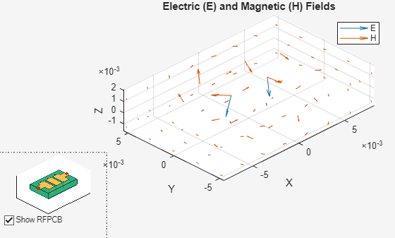
Plot the Fields

Plot the electric and magnetic fields, scaling the fields by a factor of 2.

EHfields(h, 1e6, p,ScaleFields= [2 2]);

Input Arguments

object — PCB object

rf pcb object | pcbComponent object

RF pcb object to calculate the field magnitudes, specified as an object from the catalog, or a pcbComponent object:

Example: wilkinsonSplitter

frequency — Frequency to calculate electric and magnetic fields

scalar in Hz | vector in Hz

Frequency or frequency range over which to calculate electric and magnetic fields, specified as a scalar or a vector in Hz.

Example: 70e6

Data Types: double

points — Cartesian coordinates of points in space

3-by-p matrix

Cartesian coordinates of points in space, specified as a 3-by-p matrix. p is the number of points at which to calculate the E-H field.

Example: [0 0 1]'

Data Types: double

Name-Value Arguments

Specify optional pairs of arguments as Name1=Value1,...,NameN=ValueN, where Name is the argument name and Value is the corresponding value. Name-value arguments must appear after other arguments, but the order of the pairs does not matter.

Example: ScaleFields=[2 0.5] specifies scalar values of the electric and magnetic fields

ScaleFields — Value by which to scale electric and magnetic fields

two-element vector

Value by which to scale the electric and magnetic fields, specified as a two-element vector. The first element scales the E field and the second element scales the H-field. A value of 2 doubles the relative length of either field. A value of 0.5 to halves the length of either field. A value of 0 plots either field without automatic scaling.

Example: ScaleFields=[2 0.5]

Data Types: double

ViewField — Field to display

"E" | "H"

Field to display, specified as either "E" or "H". "E" displays the electric field and "H" displays the magnetic field.

Example: ViewField="E"

Data Types: string

CoordinateSystem — Coordinate system

"rectangular" (default) | "spherical"

Coordinate system to calculate the electric and magnetic fields of a catalog component or pcbComponent object, specified as either "rectangular" or "spherical". In the Rectangular Coordinate System (Antenna Toolbox), EHfields returns the x, y, and z components of the electric and magnetic fields. In the Spherical Coordinate System (Antenna Toolbox), EHfields returns the azimuth, elevation and radial components of electric and magnetic fields.

Note

If you specify Polarization as either "H" or "V", the EHfields function uses spherical Coordinate system for calculations and output.

Example: CoordinateSystem="spherical"

Data Types: string

Polarization — Polarization of electric field

"combined" (default) | "H" | "V"

Polarization of the electric field, specified as either "H" for horizontal polarization or "V" for vertical polarization or "combined" for mixed horizontal and vertical polarization. The default value is set to "combined". The magnetic field has the opposite polarization.

When you specify Polarization as either "H" or "V" in a syntax without output arguments, the EHfields function calculates and returns the complex value of the azimuth or elevation component of the polarized electric field as a 1-by-p vector. p represents the number of points to calculate the field.

For vertical polarization, E-field is the elevation component and H-field is the azimuth component. For horizontal polarization, E-field is the azimuth component and H-field is the elevation component.

Example: Polarization="H"

Data Types: string

Output Arguments

e — Components of electrical field

3-by-p complex matrix in V/m

x, y, z components of electrical field in the rectangular coordinate system or azimuth, elevation, radial components in the spherical coordinate system, returned as 3-by-p complex matrix in V/m. The dimension p is the number of points in space at which the electric and magnetic fields are computed.

h — Components of magnetic field

3-by-p complex matrix in A/m

x, y, z components of magnetic field in the rectangular coordinate system or azimuth, elevation, radial components in the spherical coordinate system, returned as a 3-by-p complex matrix in A/m. The dimension p is the number of points in space at which the electric and magnetic fields are computed.

Version History

Introduced in R2025a