Export Labeled Data from Signal Labeler for AI-Based Spectrum Sensing Applications
The ubiquitousness of wireless devices and scarcity of licensed spectrum bands has increased the demand for efficiency in wireless spectrum usage. There are opportunities for improving the efficiency of spectrum usage beyond that afforded by conventional methods by using spectrum-sensing techniques that involve machine learning and deep learning algorithms. Spectrum sensing is an important step in cognitive radio that allows systems to determine availability of frequency resources and is also used in applications such as radar-centric integrated sensing and radar target detection and classification.
This example shows how to train both a semantic segmentation network and an object detection network for detecting RF frames using deep learning. The Signal Labeler app is used to create training labeled data from complex RF I/Q signals in the time-frequency domain. The neural networks in this example are trained to identify three different types of Bluetooth® frames, WLAN frames, and collisions between two or more types of frames.
Computer vision uses semantic segmentation and object detection techniques to identify objects and their locations in an image or video. In wireless communication and radar applications, the objects of interest are radio waveforms coming from different wireless standards, radar pulses, or unknown sources. The locations of the objects are the time and frequency regions these waveforms occupy in the time-frequency domain.
Prepare Training Data
Load Training Data
This example uses the Spectrogram Data Set for Deep Learning Based RF-Frame Detection data set [1]. The data set contains 20,000 augmented signal segments. This example uses a subset of the data set such that each signal has a random number of different Wi-Fi® and Bluetooth frames. The size of this data set is 4,831 signals.
% Define the location the dataset will be stored. By default, the temporary
% folder for the system will be used.
baseDir = tempdir;
baseDataDir = fullfile(baseDir, "SpectrogramRFFrameDetectionData");
baseNetworkDir = fullfile(baseDir, "SpectrogramRFFrameDetectionNetwork");
unzip("https://ssd.mathworks.com/supportfiles/SPT/data/SpectrogramRFFrameDetectionData.zip", ...
    baseDir);
Format Signals for Labeling in Signal Labeler
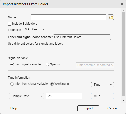
Open the Signal Labeler app by typing signalLabeler in the MATLAB command window. On the Labeler tab, click Import and select From Folders in the Members list. In the dialog box that appears, select the SpectrogramRFFrameDetectionData folder inside the temporary folder. Select MAT files in the Extension dropdown. Specify the sample rate of the dataset in the Time information section by selecting the Working in radio button. Select Time in the dropdown. Specify the sample rate as 25 MHz. Click Import.
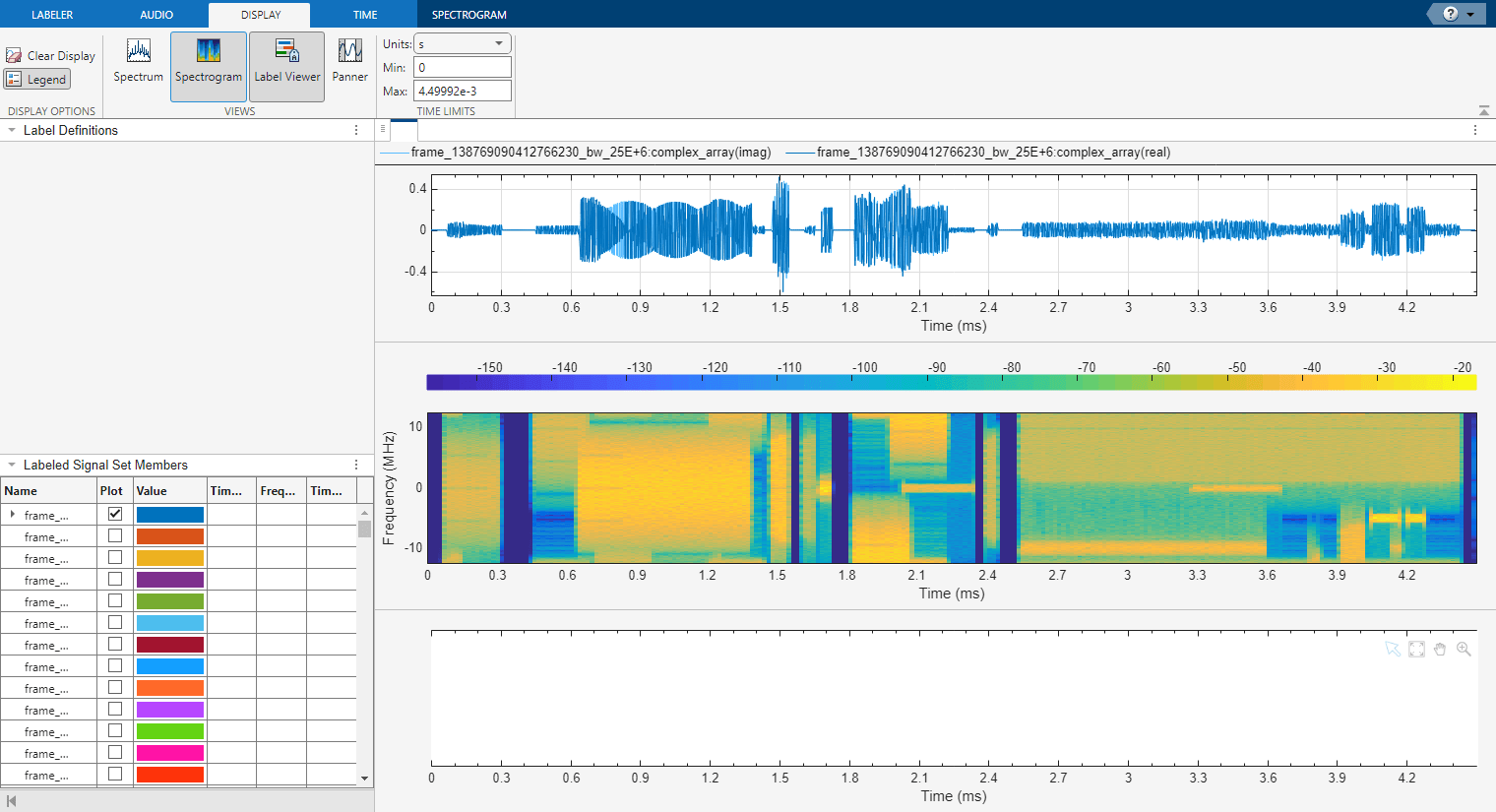
The imported files appear in the Label Signal Set Members browser.
Plot the first signal by selecting the check box next to the signal's name.
Click the Display tab, select Spectrogram in the Views section. The app displays a set of axes with the signal spectrogram and a Spectrogram tab.
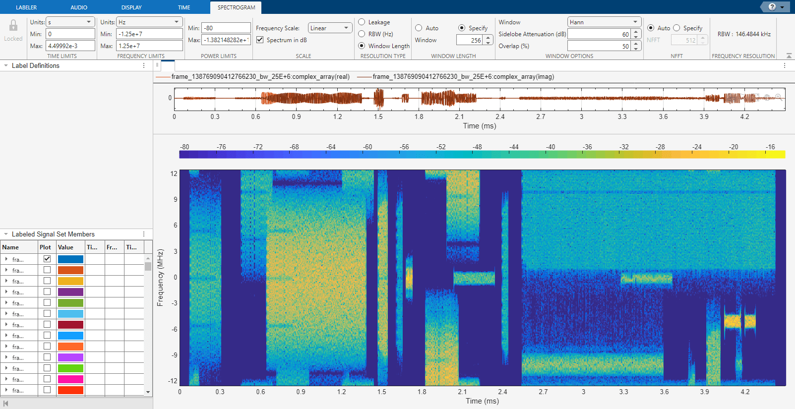
Modify the spectrogram parameters to get a clear spectrogram where the waveforms of interest are easy to identify. It is important that each waveform is clear in each member, as these settings are locked when labeling areas of interest in the app. Ensure that many members have clear waveforms by cycling through members in the toolstrip. In the Labeler tab, select the Next or Previous in the Member Navigation section.

The spectrogram settings used in this example include a Hann window of length 256, an overlap of 50%, and a minimum power limit of –80 dB. The minimum power limit reduces the power dynamic range of the spectrogram making it easier to identify regions that contain waveforms.
To label data in the Signal Labeler app, first create a label definition. Click the Labeler tab. In the Label Definition section, click the Add button to add a label definition. This label definition is used to manually label the data set. In the dialog box, name the label definition RFFrame. Set the label type to Time-Frequency ROI in the dropdown. Optionally give the label definition a description. Set the data type to categorical in the dropdown. In the categories text area, add the categories BLE_1MHz, BLE_2MHz, BT_classic, WLAN, and collision which are the labels describing three different Bluetooth waveforms, WLAN waveforms, and waveform collisions respectively.
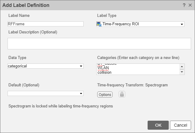
Click the Options button in the Time-frequency Transform section to inspect the spectrogram options associated with the label definition. Note that the app automatically uses the spectrogram settings that were previously set in the toolstrip while exploring some of the signals in the data set.
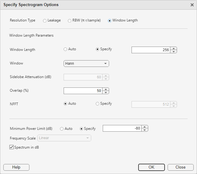
The label definition uses the specified options to create spectrograms associated with all labels, enforcing a tight connection between the I/Q signals and the spectrograms used for labeling. Click OK in the Specify Spectrogram Options dialog box to accept these settings. Click OK in the Add Label Definition dialog box to finalize the creation of the label definition.
Click OK in the information dialog box after creating a new label definition to accept that the spectrogram parameters chosen are locked while labeling.
Manually Label RF Frames in the Signal Labeler
The RFFrame label definition in the Label Definition browser is automatically selected after you create the label. Draw Labels is automatically activated.
Label the signals one at a time:
Click the spectrogram plot. A thick animated dashed line appears that expands into a shaded region when you click and drag.
Move and resize the active region until it encloses a radio signal. For better placement, you can go to the Display tab and activate the panner or choose a zoom action at the top right corner of the spectrogram plot.
Use the dropdown selector to choose the appropriate signal label definition category. The first frame has just one WLAN signal.
Check the Accept box in the Options section of the Labeler tab. Press Enter or double-click to label the time-frequency ROI. The region changes to a slight gray gradient and the outline of the region matches the member color.
Repeat the procedure in steps 1, 2, 3 and, 4 for all other radio signals in the member.
Before labeling the next member, remove the first signal from the plot by clearing the check box next to its name in the Labeled Signal Set Members browser. You cannot have two signals plotted while the spectrogram axis is active.
Plot the next member and repeat the entire procedure for each member in the data set.

Export Labeled Signal Set
Once labeling all the signals is complete export the labeled data set as a new labeledSignalSet object. You can export the labeled signal set to the MATLAB® Workspace or to a MAT file. On the Labeler tab, click Export and select To Workspace from the Labeled Signal Set list. In the dialog box that appears, give the name labeledLss to the labeled signal set, add an optional short description, and click Export. See Export Labeled Signal Sets and Signal Label Definitions for more information on how Signal Labeler exports labeled signal sets. For convenience, this example includes the resulting exported labeledSignalSet object so that it is not necessary to manually label all signals in the data set.
The next section details how to use the data and labels stored in the exported labeled signal set to train detection and segmentation deep learning models.
Train a YOLOX Object Detection Network
Load the labeled signal set. Set the AlternateFileSystemRoots to the folder location where the files were downloaded so that you can use the labeled signal set in your machine.
load(fullfile(baseDataDir,"preLabeledSignalSet.mat"));
labeledLss.setAlternateFileSystemRoots(...
    [labeledLss.Source.Folders, baseDataDir]);
Prepare Data for Training
The desired object detection network for this example uses an input image and produces regions of interest with associated labels. Each label instance describes the type of waveform detected, either BLE_1MHz, BLE_2MHz, BT_classic, WLAN, or collision.
The exported labeled signal set contains all of the signals in the data set and all the created labels. The labels have regions of interest defined by limits in both time and frequency. To train a network the signals must be converted first from the time domain into a spectrogram, and then further from a spectrogram into an image. The labels also need to be transformed from time and frequency limits to a format that the network understands. The createDatastores function of the labeledLss object helps with this process.
The target object detection network expects images of size 256 by 256 by 3. The unmodified spectrograms created by the labeledLss object will be greater than these dimensions so they will be resized to fit the image dimensions the network expects.
imageSize = [256 256];
The YOLOX network can take in rectangular regions of interest in the "Axis-aligned rectangle" format. This format is defined as spatial coordinates as an M-by-4 numeric matrix with rows of the form [x y w h], where:
M is the number of axis-aligned rectangles.
x and
yspecify the upper-left corner of the rectangle.w specifies the width of the rectangle, which is its length along the x-axis.
h specifies the height of the rectangle, which is its length along the y-axis.
The "Axis-aligned rectangle" format is used for both the training data and the detected results from the network.
To get images of the desired size and corresponding region labels use the createDatastores function of the labeldLss object. This will create a transformed datastore that generates images out of the spectrograms and an array datastore that contains the label information in the right format. Specify the TimeFrequencyMapFormat property as image to transform the spectrogram to an uint8 image. Specify the TimeFrequencyImageSize property to produce spectrogram images of size 256 by 256. To return an array datastore that has the label borders in "Axis-aligned rectangle" format, set the TimeFrequencyLabelFormat to xywh. This array datastore also contains the label values as a categorical.
labelDefinitionName = "RFFrame";
[odSds,odLds] = labeledLss.createDatastores(labelDefinitionName, ...
    TimeFrequencyLabelFormat="xywh", ...
    TimeFrequencyMapFormat="image", ...
    TimeFrequencyImageSize=[imageSize(1),imageSize(2)], ...
    TimeFrequencyIncludePartialBins=true);
The transformDatastore object odSds computes the spectrogram using the settings defined in the label definition when the read function is called. The spectrogram is transformed into a three-dimensional image whose first two dimensions are specified by imageSize.
The arrayDatastore object odLds contains the label information in the "Axis-aligned rectangle" form that has been mapped to the dimensions specified by imageSize. These label values stored in odLds are transformed from the time and frequency limits seen in the labeledLss object to pixel values of the resized spectrogram.
Inspect Labels
Inspect the first spectrogram and its associated labels within the datastores. For each label, plot the boundaries of the label as a rectangle and label the rectangle with the label value.
Get the first spectrogram image and its associated labels.
[specImage, specInfo] = odSds.read;
odSds.reset;
specLabel = odLds.preview;
Plot the image of the spectrogram specImage.
imagesc(specImage);
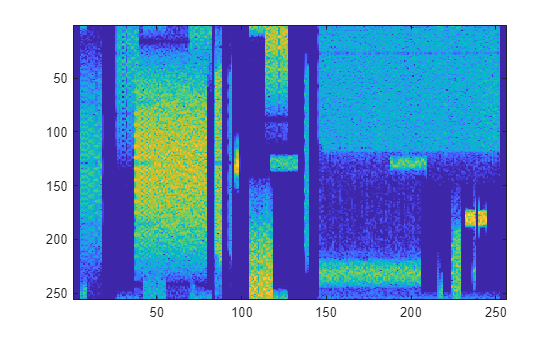
The struct specInfo contains the information required to display the axes limits and ticks, as well as the options used to create the spectrogram from the time domain signal.
The locations of the labels and the values of the labels are stored in the cell array specLabel.
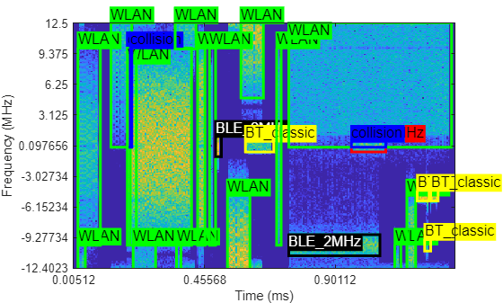
Plot the spectrogram image and the associated labels with the helperObjectDetectionPlotter function.
catsObjectDetection = ["BLE_1MHz" "BLE_2MHz" "BT_classic" "WLAN" "collision"];
helperObjectDetectionPlotter(specImage,specInfo,specLabel,catsObjectDetection);
Split Training, Validation, and Test Sets
Split the data sets into training, validation, and test sets. Allocate 80% of the data for training, 10% for validation, and 10% for test. Use a random number stream for repeatability of the shuffled order of files.
parts = [80 10 10];
s = RandStream("mt19937ar",Seed=0);
numFiles = labeledLss.NumMembers;
shuffledIndices = randperm(s,numFiles);

numTrain = floor(numFiles*parts(1)/100);
numVal = floor(numFiles*parts(2)/100);

odSdsTrain = subset(odSds,shuffledIndices(1:numTrain));
odSdsVal = subset(odSds,shuffledIndices(numTrain+(1:numVal)));
odSdsTest = subset(odSds,shuffledIndices(numTrain+numVal+1:end));

odLdsTrain = subset(odLds,shuffledIndices(1:numTrain));
odLdsVal = subset(odLds,shuffledIndices(numTrain+(1:numVal)));
odLdsTest = subset(odLds,shuffledIndices(numTrain+numVal+1:end));
Combine the datastores containing the spectrogram and the label information into a single datastore for training.
odCdsTrain = combine(odSdsTrain,odLdsTrain);
odCdsVal = combine(odSdsVal,odLdsVal);
odCdsTest = combine(odSdsTest,odLdsTest);
Train Deep Neural Network for Object Detection
This example uses the YOLOX object model for the detection problem because it is suited for quickly identifying waveforms in input spectrograms. The YOLOX model is a single-stage, anchor-free technique, which significantly reduces the model size and improves computation speed compared to previous YOLO models. Instead of using memory-intensive predefined anchor boxes, YOLOX localizes objects directly by finding object centers.
For this example, you can train a network which could take up to several hours or you can use a pretrained network provided with the data. You can skip the training step by downloading the pretrained network detector using the selector below. To train the network as the example runs, set trainNow to true. To skip the training steps and download a MAT file containing the pretrained network, set trainNow to false.
trainNow =false; if trainNow frameDetector = yoloxObjectDetector("tiny-coco",catsObjectDetection, ... InputSize=[imageSize(1),imageSize(2),3]); end
Configure training using the trainOptions (Deep Learning Toolbox) function to specify the stochastic descent with momentum (SGDM) optimization algorithm and the hyper-parameters used for SGDM. Train the object detector for a maximum of 100 epochs. Specify the ValidationData name-value argument as the validation data as odCdsVal. Set OutputNetwork to "best-validation-loss" to obtain the network with the lowest validation loss during training when the training finishes.
options = trainingOptions("sgdm", ...
    InitialLearnRate=5e-4, ...
    LearnRateSchedule="piecewise", ...
    LearnRateDropFactor=0.99, ...
    LearnRateDropPeriod=1, ...
    MiniBatchSize=20, ...
    MaxEpochs=100, ...
    ExecutionEnvironment="auto", ...
    Shuffle="every-epoch", ...
    VerboseFrequency=25, ...
    ValidationFrequency=100, ...
    ValidationData=odCdsVal, ...
    ResetInputNormalization=false, ...
    OutputNetwork="best-validation-loss", ...
    GradientThreshold=30, ...
    L2Regularization=5e-4);
Train the detector by using the trainYOLOXObjectDetector (Computer Vision Toolbox)function.
if trainNow
    frameDetector = trainYOLOXObjectDetector(cdsTrain,frameDetector, ...
        options,"FreezeSubNetwork","none");
    modelDateTime = string(datetime("now",Format="yyyy-MM-dd-HH-mm-ss"));
    save(fullfile(baseNetworkDir,"trainedRFFrameDetectorYoloX"+modelDateTime), ...
        "frameDetector")
else
    load(fullfile(baseNetworkDir,"networks.mat"),"frameDetector");
end
Evaluate Detector
Detect the bounding boxes for all test images. Set the detection threshold to a low value to detect as many objects as possible and evaluate the detection performance across a full range of detection score values.
detectionThresh = 0.1;
detectorResults = detect(frameDetector,odCdsTest, ...
    AutoResize=false,MiniBatchSize=1,Threshold=detectionThresh);
Calculate object detection metrics on the test set detection results by using the evaluateObjectDetection (Computer Vision Toolbox) function on the test partition of the data set.
metricsObjectDetection = evaluateObjectDetection(detectorResults,odCdsTest);
Calculate and display the average precision (AP) score for each class. Average precision quantifies the ability of the detector to classify objects correctly.
AP = averagePrecision(metricsObjectDetection);
disp(table(catsObjectDetection',AP,VariableNames=["Category","AP"]));
      Category        AP
    ____________    _______

    "BLE_1MHz"      0.85924
    "BLE_2MHz"      0.81538
    "BT_classic"     0.6855
    "WLAN"          0.86357
    "collision"     0.24459
The detector performs well in detecting the Bluetooth and Wi-Fi frames but struggles to capture areas of collision correctly. This is expected as collisions make it harder to determine the correct signal types and regions over where the signals are present.
Evaluate Detector Errors Using Confusion Matrix
The confusion matrix helps quantify the performance of the detector object across different classes by providing a detailed breakdown of the detection errors. Investigate the types of classification errors made by the detector at a selected detection score threshold by using the confusionMatrix (Computer Vision Toolbox) object function. Use the detection score threshold you determined from the precision recall analysis to discard predictions below that threshold value.
Compute the confusion matrix at a specified score.
[confMat,confusionClassNames] = confusionMatrix(metricsObjectDetection, ...
    scoreThreshold=detectionThresh);
Display the confusion matrix as a confusion chart.
figure
confusionchart(confMat{1},confusionClassNames)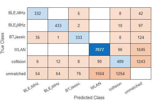
The results show the network can accurately predict areas in the spectrogram image that contain WLAN and Bluetooth 1 and 2 MHz signals. The network does not classify the collision between two signals well.
Train a Semantic Segmentation Network
Prepare Data for Training
Semantic segmentation networks assign a value to every pixel of the input image. The network trained in this example assigns values based on the type of waveform detected, either BLE_1MHz, BLE_2MHz, BT_classic, WLAN, collision, or no waveform detected. Both the data used to train the network and the output of the trained network use this format.
Add a category to the labeled signal set to utilize the sixth label type that represents no waveform detected.
catsSemanticSegmentation = ["BLE_1MHz","BLE_2MHz","BT_classic","WLAN", ...
    "collision","undefined"];
labeledLss.editLabelDefinition(labelDefinitionName, ...
    Categories=catsSemanticSegmentation);
This example utilizes transfer learning on a few existing networks shipped with MATLAB. The resne18, resnet50, and mobilenetv2 models all require input image sizes of at least 224 by 224. In this example the image dimensions are constrained to 256 by 256 by 3 to meet this criterion. Adjust the image size to see changes in training speed and overall performance.
imageSize = [256,256];
The labels used to train the network need to match the size of the spectrogram image. For each spectrogram image, you must create a categorical array of the same size as the image. Each value within the categorical array corresponds to a single pixel in the spectrogram image.
Use the createDatastores object function of the labeldLss object to create a transformed datastore that contains a signal datastore and an array datastore that contains the label information expected by the network for training a semantic segmentation problem. Specify the TimeFrequencyMapFormat property as image to return an uint8 image. Specify the TimeFrequencyImageSize property to ensure the transformed datastore returns an image of the spectrogram of size 256 by 256. To return an array datastore that has the label borders as a categorical array of the same dimension as the spectrogram image, set the TimeFrequencyLabelFormat to "mask".
[ssSds,ssLds] = labeledLss.createDatastores(labelDefinitionName, ...
    TimeFrequencyLabelFormat="mask", ...
    TimeFrequencyMapFormat="image", ...
    TimeFrequencyImageSize=[imageSize(1) imageSize(2)], ...
    TimeFrequencyIncludePartialBins=true);
Transform the array datastore that contains the labels with the transform method and the included replaceUnknowns helper function. This function replaces any missing data values returned by the datastore with the sixth category in the label definition, "undefined".
ssLds = transform(ssLds,@replaceUnknowns);
Inspect Labels
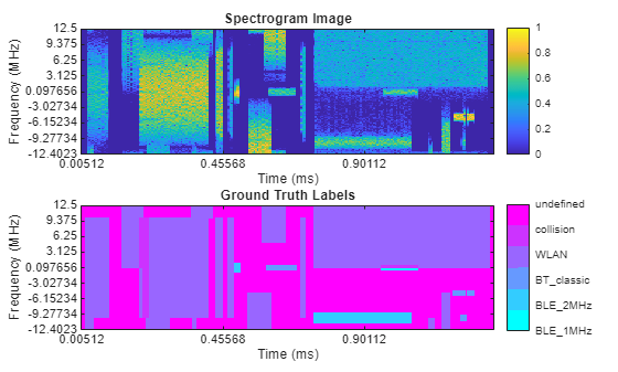
Inspect the first spectrogram and associated labels within the datastores. Plot the spectrogram as well as an image the same size as the spectrogram with the mask areas identified.
Get the first spectrogram and its associated labels.
[specImage, specInfo] = ssSds.read;
ssSds.reset;
specLabel = ssLds.preview;
Plot the spectrogram as an image using the helperSemanticSegmentationPlotter helper function.
helperSemanticSegmentationPlotter(specImage,specInfo,specLabel,catsSemanticSegmentation)
Prepare Training, Validation and Test Sets
Split the data sets into training, validation and test sets. Allocate 80% of the data for training, 10% for validation and 10% for test. Use a random number stream for repeatability of the shuffled order of files.
parts = [80 10 10];
s = RandStream("mt19937ar",Seed=0);
numFiles = labeledLss.NumMembers;
shuffledIndices = randperm(s,numFiles);

numTrain = floor(numFiles*parts(1)/100);
numVal = floor(numFiles*parts(2)/100);

ssSdsTrain = subset(ssSds,shuffledIndices(1:numTrain));
ssSdsVal = subset(ssSds,shuffledIndices(numTrain+(1:numVal)));
ssSdsTest = subset(ssSds,shuffledIndices(numTrain+numVal+1:end));

ssLdsTrain = subset(ssLds,shuffledIndices(1:numTrain));
ssLdsVal = subset(ssLds,shuffledIndices(numTrain+(1:numVal)));
ssLdsTest = subset(ssLds,shuffledIndices(numTrain+numVal+1:end));
Combine the datastores containing the spectrogram and the label information into a single combined datastore for training.
ssCdsTrain = combine(ssSdsTrain,ssLdsTrain);
ssCdsVal = combine(ssSdsVal,ssLdsVal);
ssCdsTest = combine(ssSdsTest,ssLdsTest);
Balance Classes Using Class Weighting
Use class weighting to improve the training when classes in the training set are not balanced. Use computed pixel label counts with the countEachPixelLabel helper function to calculate the median frequency class weights.
tbl = countEachPixelLabel(ssLdsTrain);
numClasses = numel(catsSemanticSegmentation);
imageFreq = tbl.PixelCount./tbl.ImagePixelCount;
classWeights = median(imageFreq)./imageFreq;
classWeights = classWeights/(sum(classWeights)+eps(class(classWeights)));
if length(classWeights) < numClasses
    classWeights = [classWeights;zeros(numClasses-length(classWeights),1)];
end
Select Training Options
Configure training with the trainingOptions (Deep Learning Toolbox) function.
mbs = 40;
opts = trainingOptions("sgdm", ...
    MiniBatchSize = mbs, ...
    MaxEpochs = 20, ...
    LearnRateSchedule = "piecewise", ...
    InitialLearnRate = 0.02, ...
    LearnRateDropPeriod = 10, ...
    LearnRateDropFactor = 0.1, ...
    ValidationData = ssCdsVal, ...
    ValidationPatience = 5, ...
    Shuffle="every-epoch", ...
    OutputNetwork = "best-validation-loss", ...
    Plots = "training-progress");
Train Deep Neural Network for Semantic Segmentation
Train the network using the combined training data store, ssCdsStore. The combined training data store contains spectrogram images and true pixel labels. Use weighted cross-entropy loss together with a custom normalization to update the network during training. Define a custom loss function, lossFunction, using the crossentropy (Deep Learning Toolbox) (Deep Learning Toolbox) loss function and apply custom normalization.
For this example, you can train a network which could take up to several hours or you can use a pretrained network provided with the data. You can skip the training by downloading the pretrained network net using the selector below. To train the network as the example runs, set trainNow to true. To skip the training steps and download a MAT file containing the pretrained network, set trainNow to false.
trainNow =false; baseNetwork =
"resnet50"; layers = deeplabv3plus([imageSize(1),imageSize(2)], ... numel(catsSemanticSegmentation),baseNetwork); if trainNow [frameSegmenter,trainInfo] = trainnet(ssCdsTrain,layers, ... @(ypred,ytrue) lossFunction(ypred,ytrue,classWeights),opts); modelDateTime = string(datetime("now",Format="yyyy-MM-dd-HH-mm-ss")); save(fullfile(baseNetworkDir,"trainedRFFrameSemanticSegmenter"+modelDateTime+".mat"), ... "frameSegmenter", "trainInfo"); else load(fullfile(baseNetworkDir, "networks.mat"), "frameSegmenter"); end
Evaluate Neural Network
Test the network signal identification performance using the test datastore ssSdsTest. Use the semanticseg (Computer Vision Toolbox) (Computer Vision Toolbox) function to get the pixel estimates of the spectrogram images in the test datastore. Use the evaluateSemanticSegmentation (Computer Vision Toolbox) (Computer Vision Toolbox) function to compute various metrics to evaluate the quality of the semantic segmentation results.
ldsPredictedResults = semanticseg(ssSdsTest, frameSegmenter, ...
    MiniBatchSize=mbs, ...
    WriteLocation=tempdir, ...
    Classes=catsSemanticSegmentation);
Running semantic segmentation network
-------------------------------------
* Processed 484 images.
metricsSemanticSeg = evaluateSemanticSegmentation(ldsPredictedResults, ssLdsTest);
Evaluating semantic segmentation results
----------------------------------------
* Selected metrics: global accuracy, class accuracy, IoU, weighted IoU, BF score.
* Processed 484 images.
* Finalizing... Done.
* Data set metrics:

    GlobalAccuracy    MeanAccuracy    MeanIoU    WeightedIoU    MeanBFScore
    ______________    ____________    _______    ___________    ___________

       0.83011          0.90123       0.59601      0.75272        0.71357
Plot the normalized confusion matrix for all test frames.
figure
cm = confusionchart(metricsSemanticSeg.ConfusionMatrix.Variables, ...
    catsSemanticSegmentation,Normalization="row-normalized")
cm =
  ConfusionMatrixChart with properties:

    NormalizedValues: [6×6 double]
         ClassLabels: ["BLE_1MHz"    "BLE_2MHz"    "BT_classic"    "WLAN"    "collision"    "undefined"]

  Show all properties
cm.Title = "Confusion Matrix - Synthetic";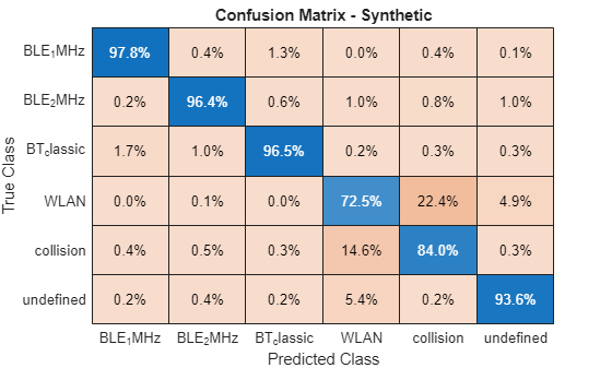
The results are accurate in correctly identifying each of three Bluetooth classes.
Plot Results of Network Segmentation
Inspect the first spectrogram and associated labels within the datastores. Plot the spectrogram as well as the mask.
Get the first spectrogram and its associated labels.
[specImage, specInfo] = ssSdsTest.read;
ssSdsTest.reset;
predictedSpecLabel = ldsPredictedResults.preview;
actualSpecLabel = ssLdsTest.preview;
Plot the spectrogram image using the helperSpectrumSensingPredictedPlotter helper function.
helperSpectrumSensingPredictedPlotter(specImage,specInfo, ...
    predictedSpecLabel,actualSpecLabel,catsSemanticSegmentation);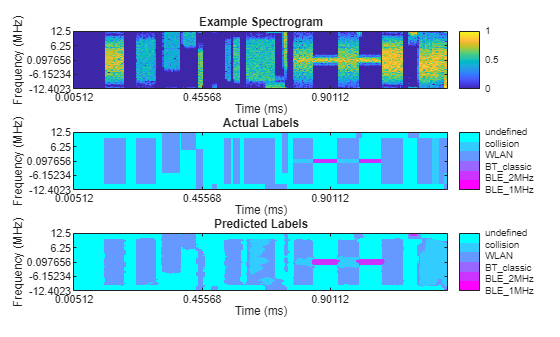
This visualization shows that the model finds sections within WLAN signals as collisions, even when no collision between signals exists. The model has a hard time differentiating overlapping WLAN signals with collision. The model does a good job detecting signals from undefined noise and retains much of the shape of the ground-truth labels.
Creating Stored Data Set
An alternate method to run this example is to save the spectrograms to files. This method has the advantage that the spectrogram images only need to be computed once. The training is done with the stored images.
Export a data set from the Signal Labeler app. Select the Create Data Set button in the Labeler tab. In the dialog box select the directory where the data set will be created. For targeting object detection problems, select [x y w h] for the Labels Format. For targeting semantic segmentation problems, select Mask. Choose a desired image size and click Create.
After the data set is created, create a signal datastore for the spectrograms and the labels.
Inspect the READ file in the exported dataset location. The variable names inside each MAT file are given in this file.
To create a signalDatastore for training a semantic segmentation problem, use the timeFrequencyMap and maskLabels variables.
% semanticSegmentationDataSetDatastore = signalDatastore(fullfile(cd, "*.mat"), ...
%     SampleRate=25e6, SignalVariableNames=["timeFrequencyMap", "maskLabels"]);
To create a datastore for training an object detection problem, use the timeFrequencyMap and the axisAlignedRectangleLabels variables. The label locations and values are stored in a cell array. To properly organize the datastores such that the read method returns a 1-by-3 cell array, use the transform method of the datastore such that the first cell contains the spectrogram image, the second cell contains the label region limits in "Axis-aligned rectangular" format, and the third cell contains a vector of the label values.
% objectDetectionDataSetDatastore = signalDatastore(...
%     fullfile(cd, "exportedDataset", "*.mat"), ...
%     SignalVariableName=["timeFrequencyMap","axisAlignedRectangleLabels"], ...
%     ReadOutputOrientation="row");
% objectDetectionDataSetDatastore = transform(@(x) [a(1), a{2}], ...
%     objectDetectionDataSetDatastore);
Both datastore objects can be used in this state to train networks with the trainnet function and trainYOLOXObjectDetector function, as shown in previous sections of this example.
Conclusions
This example shows how to use the Signal Labeler app to label time-frequency regions of the signal spectrograms. The resulting labeled data set can be used to train object detection and semantic segmentation models.
Manually labeling on top of spectrograms can take a long time on larger datasets. To expedite this process, consider the following example: Automated Labeling of Time-Frequency Regions for AI-Based Spectrum Sensing Applications.
Supporting Functions
function helperObjectDetectionPlotter(specImage, specInfo, specLabel, categories)
    hFig = figure;
    hAx = axes(hFig);
    image(specImage,"Parent",hAx);

    % Use the specInfo output from the transformed datastore to assign tick labels
    % on the x and y axes.
    yidx = linspace(1,size(specInfo.Frequencies,1),9);
    yticks(hAx, yidx);
    yticklabels(hAx, flipud(string(specInfo.Frequencies(round(yidx))/1e6)));
    ylabel(hAx, "Frequency (MHz)");

    xidx = linspace(1, size(specInfo.Time,2),11);
    xticks(hAx, xidx);
    xticklabels(hAx, string(specInfo.Time(round(xidx))*1e3));
    xlabel(hAx, "Time (ms)");

    % Draw a rectangle on the axis for each label. Assign the associated label
    % and color by label value.
    categoryColors = ["red","k","yellow","green","blue","magenta"];
    for i = 1:numel(specLabel{2})
        hR = drawrectangle(hAx, "Position", specLabel{1}(i,:));
        hR.InteractionsAllowed = "none";
        hR.Label = string(specLabel{2}(i));
        hR.Color = categoryColors(hR.Label == categories);
        hR.FaceAlpha = 0;
    end
end

function helperSemanticSegmentationPlotter(specImage, specInfo, specLabel, ...
    categories)
    figure;
    hAx = subplot(211);
    image(specImage,"Parent",hAx);

    % Use the specInfo output from the transformed datastore to assign tick label
    % on the x and y axes.
    yidx = linspace(1,size(specInfo.Frequencies,1),9);
    yticks(hAx, yidx);
    yticklabels(hAx, flipud(string(specInfo.Frequencies(round(yidx))/1e6)));
    ylabel(hAx, "Frequency (MHz)");

    xidx = linspace(1, size(specInfo.Time,2),11);
    xticks(hAx, xidx);
    xticklabels(hAx, string(specInfo.Time(round(xidx))*1e3));
    xlabel(hAx, "Time (ms)");

    % Add a colorbar.
    colorbar;

    title("Spectrogram Image");

    % Draw the label output mask.
    hAx = subplot(212);
    labelValues = double(specLabel{1});
    im = imagesc(labelValues, [1 numel(categories)]);

    % Use the specInfo output from the transformed datastore to assign tick labels
    % on the x and y axes.
    yidx = linspace(1,size(specInfo.Frequencies,1),9);
    yticks(hAx, yidx);
    yticklabels(hAx, flipud(string(specInfo.Frequencies(round(yidx))/1e6)));
    ylabel(hAx, "Frequency (MHz)");

    xidx = linspace(1, size(specInfo.Time,2),11);
    xticks(hAx, xidx);
    xticklabels(hAx, string(specInfo.Time(round(xidx))*1e3));
    xlabel(hAx, "Time (ms)");

    % Add a colorbar that identifies the label category by color.
    cmap = cool(numel(categories));
    ticks = 1:numel(categories);

    im.Parent.Colormap = cmap;
    colorbar(TickLabels=cellstr(categories),Ticks=ticks,...
        TickLength=0,TickLabelInterpreter="none");

    title("Ground Truth Labels");
end

function helperSpectrumSensingPredictedPlotter(specImage, specInfo, ...
    predictedSpecLabel, actualSpecLabel, categories)
    figure;
    hAx = subplot(311);
    image(specImage,"Parent",hAx);
    title("Example Spectrogram");

    % Use the specInfo output from the transformed datastore to assign tick labels on
    % the x and y axes.
    yidx = linspace(1,size(specInfo.Frequencies,1),5);
    yticks(hAx, yidx);
    yticklabels(hAx, flipud(string(specInfo.Frequencies(round(yidx))/1e6)));
    ylabel(hAx, "Frequency (MHz)");

    xidx = linspace(1, size(specInfo.Time,2),11);
    xticks(hAx, xidx);
    xticklabels(hAx, string(specInfo.Time(round(xidx))*1e3));
    xlabel(hAx, "Time (ms)");

    % Add a colorbar.
    colorbar;

    % Draw the actual label mask.
    hAx = subplot(312);
    labelValues = double(actualSpecLabel{1});
    im = imagesc(labelValues, [1 numel(categories)]);
    title("Actual Labels");

    % Use the specInfo output from the transformed datastore to assign tick labels on
    % the x and y axes.
    yidx = linspace(1,size(specInfo.Frequencies,1),5);
    yticks(hAx, yidx);
    yticklabels(hAx, flipud(string(specInfo.Frequencies(round(yidx))/1e6)));
    ylabel(hAx, "Frequency (MHz)");

    xidx = linspace(1, size(specInfo.Time,2),11);
    xticks(hAx, xidx);
    xticklabels(hAx, string(specInfo.Time(round(xidx))*1e3));
    xlabel(hAx, "Time (ms)");

    % Add a colorbar that identifies the label category by color.
    cmap = cool(numel(categories));
    ticks = 1:numel(categories);

    im.Parent.Colormap = flipud(cmap);
    colorbar(TickLabels=cellstr(categories),Ticks=ticks,...
        TickLength=0,TickLabelInterpreter="none");

    % Draw the predicted label mask.
    hAx = subplot(313);
    labelValues = double(predictedSpecLabel);
    im = imagesc(labelValues, [1 numel(categories)]);
    title("Predicted Labels");

    % Use the specInfo output from the transformed datastore to assign tick labels on
    % the x and y axes.
    yidx = linspace(1,size(specInfo.Frequencies,1),5);
    yticks(hAx, yidx);
    yticklabels(hAx, flipud(string(specInfo.Frequencies(round(yidx))/1e6)));
    ylabel(hAx, "Frequency (MHz)");

    xidx = linspace(1, size(specInfo.Time,2),11);
    xticks(hAx, xidx);
    xticklabels(hAx, string(specInfo.Time(round(xidx))*1e3));
    xlabel(hAx, "Time (ms)");

    % Add a colorbar that identifies the label category by color.
    cmap = cool(numel(categories));
    ticks = 1:numel(categories);

    im.Parent.Colormap = flipud(cmap);
    colorbar(TickLabels=cellstr(categories),Ticks=ticks,...
        TickLength=0,TickLabelInterpreter="none");
end

function [labelsOut, info] = replaceUnknowns(dataIn, info)
    % This function replaces the missing values of a categorical array with
    % the string "undefined".
    missingLabels = ismissing(dataIn{1});
    labels = dataIn{1};
    labels(missingLabels) = "undefined";
    labelsOut = {labels};
end

function tbl = countEachPixelLabel(lds)
    labels = lds.read();
    lds.reset();
    labels = labels{1};

    % Initialize counter
    cats = categories(labels(1));
    s = struct();
    for i = 1:numel(cats)
        s.(cats{i}) = 0;
    end
    st = s;

    labels = lds.readall();
    for i = 1:numel(labels)
        label = labels{i};
        for j = 1:numel(cats)
            cat = cats{j};
            numPixels = sum(label(:) == cat);
            s.(cat) = s.(cat) + numPixels;
            if (numPixels) > 0
                st.(cat) = st.(cat) + numel(label(:));
            end
        end
    end

    tbl = table(cats, zeros(numel(cats),1), zeros(numel(cats),1),...
        VariableNames=["Name","PixelCount","ImagePixelCount"]);
    for i = 1:numel(cats)
        tbl.PixelCount(i) = s.(cats{i});
        tbl.ImagePixelCount(i) = st.(cats{i});
    end
end

function loss = lossFunction(ypred,yactual,weights)
    % Compute weighted cross-entropy loss.
    cdim = strfind(dims(ypred), "C");
    loss = crossentropy(ypred,yactual,weights,WeightsFormat="C", ...
        NormalizationFactor="none");
    wn = shiftdim(weights(:)',-(cdim-2));
    wnT = extractdata(yactual).*wn;
    normFac = sum(wnT(:))+eps("single");
    loss = loss/normFac;
end
References
[1] Wicht, J., Wetzker, U., & Jain, V. (2022). Spectrogram Data Set for Deep-Learning-Based RF Frame Detection. Data, 7(12), 168. https://doi.org/10.3390/data7120168
See Also
Apps
Functions
Objects
labeledSignalSet|yoloxObjectDetector(Computer Vision Toolbox)