Mark Signals of Interest for Control System Analysis and Design

Analysis Points

Whether you model your control system in MATLAB^® or Simulink^®, use analysis points to mark points of interest in the model. Analysis points allow you to access internal signals, perform open-loop analysis, or specify requirements for controller tuning. In the block diagram representation, an analysis point can be thought of as an access port to a signal flowing from one block to another. In Simulink, analysis points are attached to the outports of Simulink blocks. For example, in the following model, the reference signal, r, and the control signal, u, are analysis points that originate from the outputs of the setpoint and C blocks respectively.

Each analysis point can serve one or more of the following purposes:

Input — The software injects an additive input signal at an analysis point, for example, to model a disturbance at the plant input.
Output — The software measures the signal value at a point, for example, to study the impact of a disturbance on the plant output.
Loop Opening — The software inserts a break in the signal flow at a point, for example, to study the open-loop response at the plant input.

You can apply these purposes concurrently. For example, to compute the open-loop response from u to y, you can treat u as both a loop opening and an input. When you use an analysis point for more than one purpose, the software applies the purposes in this sequence: output measurement, then loop opening, then input.

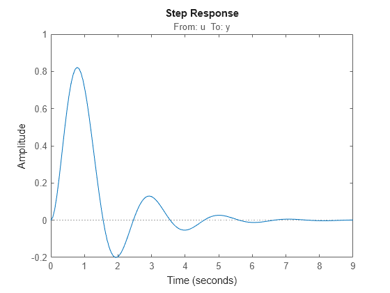
Using analysis points, you can extract open-loop and closed-loop responses from a control system model. For example, suppose T represents the closed-loop system in the model above, and u and y are marked as analysis points. T can be either a generalized state-space model or an slLinearizer or slTuner interface to a Simulink model. You can plot the closed-loop response to a step disturbance at the plant input with the following commands:

Tuy = getIOTransfer(T,'u','y');
stepplot(Tuy)

Analysis points are also useful to specify design requirements when tuning control systems with the systune command. For example, you can create a requirement that attenuates disturbances at the plant input by a factor of 10 (20 dB) or more.

Req = TuningGoal.Rejection('u',10);

Specify Analysis Points for MATLAB Models

Consider an LTI model of the following block diagram.

G = tf(10,[1 3 10]);
C = pid(0.2,1.5);
T = feedback(G*C,1);

With this model, you can obtain the closed-loop response from r to y. However, you cannot analyze the open-loop response at the plant input or simulate the rejection of a step disturbance at the plant input. To enable such analysis, mark the signal u as an analysis point by inserting an AnalysisPoint block between the plant and controller.

AP = AnalysisPoint('u');
T = feedback(G*AP*C,1);
T.OutputName = 'y';

The plant input, u, is now available for analysis.

In creating the model T, you manually created the analysis point block AP and explicitly included it in the feedback loop. When you combine models using the connect command, you can instruct the software to insert analysis points automatically at the locations you specify. For more information, see connect.

Specify Analysis Points for Simulink Models

In Simulink, you can mark analysis points either explicitly in the block diagram, or programmatically using the addPoint command for slLinearizer or slTuner interfaces.

To specify analysis points directly in your Simulink model, first open the Linearization tab. To do so, in the Apps gallery, click Linearization Manager.

To specify an analysis point:

In the model, click the signal you want to define as an analysis point.
On the Linearization tab, in the Insert Analysis Points gallery, select the type of analysis point you want to define.
When you specify analysis points, the software adds annotations to your model indicating the linear analysis point type.
Repeat steps 1 and 2 for all signals you want to define as analysis points.

You can select any of the following closed-loop analysis point types, which are equivalent within an slLinearizer or slTuner interface; that is, they are treated the same way by analysis functions, such as getIOTransfer, and tuning goals, such as TuningGoal.StepTracking.

Input Perturbation
Output Measurement
Sensitivity
Complementary Sensitivity

If you want to introduce a permanent loop opening at a signal as well, select one of the following open-loop analysis point types:

Open-Loop Input
Open-Loop Output
Loop Transfer
Loop Break

When you define a signal as an open-loop point, analysis functions such as getIOTransfer always enforce a loop break at that signal during linearization. All open-loop analysis point types are equivalent within an slLinearizer or slTuner interface. For more information on how the software treats loop openings during linearization, see How the Software Treats Loop Openings.

When you create an slLinearizer or slTuner interface for a model, any analysis points defined in the model are automatically added to the interface. If you defined an analysis point using:

A closed-loop type, the signal is added as an analysis point only.
An open-loop type, the signal is added as both an analysis point and a permanent opening.

To mark analysis points programmatically, use the addPoint command. For example, consider the scdcascade model.

open_system('scdcascade')

To mark analysis points, first create an slTuner interface.

ST = slTuner('scdcascade');

To add a signal as an analysis point, use the addPoint command, specifying the source block and port number for the signal.

addPoint(ST,'scdcascade/C1',1);

If the source block has a single output port, you can omit the port number.

addPoint(ST,'scdcascade/G2');

For convenience, you can also mark analysis points using the:

Name of the signal.
```
addPoint(ST,'y2');
```
Combined source block path and port number.
```
addPoint(ST,'scdcascade/C1/1')
```
End of the full source block path when unambiguous.
```
addPoint(ST,'G1/1')
```

You can also add permanent openings to an slLinearizer or slTuner interface using the addOpening command, and specifying signals in the same way as for addPoint. For more information on how the software treats loop openings during linearization, see How the Software Treats Loop Openings.

addOpening(ST,'y1m');

You can also define analysis points by creating linearization I/O objects using the linio command.

io(1) = linio('scdcascade/C1',1,'input');
io(2) = linio('scdcascade/G1',1,'output');
addPoint(ST,io);

As when you define analysis points directly in your model, if you specify a linearization I/O object with:

A closed-loop type, the signal is added as an analysis point only.
An open-loop type, the signal is added as both an analysis point and a permanent opening.

When you specify response I/Os in a tool such as Model Linearizer or Control System Tuner, the software creates analysis points as needed.

Refer to Analysis Points for Analysis and Tuning

Once you have marked analysis points, you can analyze the response at any of these points using the following analysis functions:

getIOTransfer — Transfer function for specified inputs and outputs
getLoopTransfer — Open-loop transfer function from an additive input at a specified point to a measurement at the same point
getSensitivity — Sensitivity function at a specified point
getCompSensitivity — Complementary sensitivity function at a specified point

You can also create tuning goals that constrain the system response at these points. The tools to perform these operations operate in a similar manner for models created at the command line and models created in Simulink.

To view the available analysis points, use the getPoints function. You can view the analysis for models created:

At the command line:
In Simulink:

For closed-loop models created at the command line, you can also use the model input and output names when:

Computing a closed-loop response.

ioSys = getIOTransfer(T,'u','y');
stepplot(ioSys)

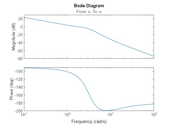
Computing an open-loop response.

loopSys = getLoopTransfer(T,'u',-1);
bodeplot(loopSys)

Creating tuning goals for systune.
```
R = TuningGoal.Margins('u',10,60);
```

Use the same method to refer to analysis points for models created in Simulink. In Simulink models, for convenience, you can use any unambiguous abbreviation of the analysis point names returned by getPoints.

ioSys = getIOTransfer(ST,'u1','y1');
sensG2 = getSensitivity(ST,'G2');
R = TuningGoal.Margins('u1',10,60);

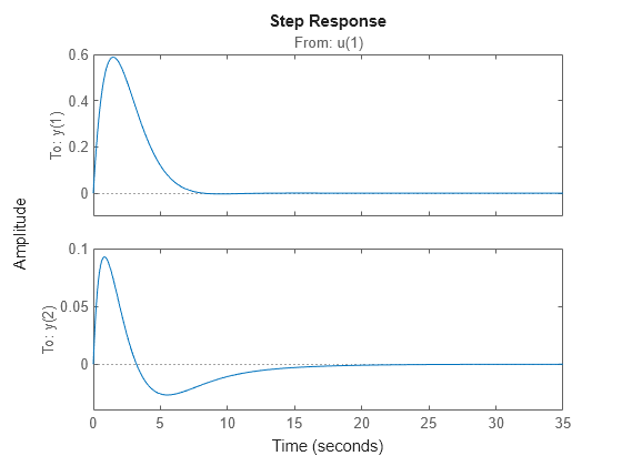
Finally, if some analysis points are vector-valued signals or multichannel locations, you can use indices to select particular entries or channels. For example, suppose u is a two-entry vector in a closed-loop MIMO model.

G = ss([-1 0.2;0 -2],[1 0;0.3 1],eye(2),0);
C = pid(0.2,0.5);
AP = AnalysisPoint('u',2);
T = feedback(G*AP*C,eye(2));
T.OutputName = 'y';

You can compute the open-loop response of the second channel and measure the impact of a disturbance on the first channel.

L = getLoopTransfer(T,'u(2)',-1);
stepplot(getIOTransfer(T,'u(1)','y'))

When you create tuning goals in Control System Tuner, the software creates analysis points as needed.