Fit Distributions to Grouped Data Using ksdensity

This example shows how to fit kernel distributions to grouped sample data using the ksdensity function.

Step 1. Load sample data.

Load the sample data.

load carsmall

The data contains miles per gallon (MPG) measurements for different makes and models of cars, grouped by country of origin (Origin), model year (Model_Year), and other vehicle characteristics.

Step 2. Group sample data by origin.

Group the MPG data by origin (Origin) for cars made in the USA, Japan, and Germany.

Origin = categorical(cellstr(Origin));
MPG_USA = MPG(Origin=='USA');
MPG_Japan = MPG(Origin=='Japan');
MPG_Germany = MPG(Origin=='Germany');

Step 3. Compute and plot the pdf.

Compute and plot the pdf for each group.

[fi,xi] = ksdensity(MPG_USA);
plot(xi,fi,'r-')
hold on

[fj,xj] = ksdensity(MPG_Japan);
plot(xj,fj,'b-.')

[fk,xk] = ksdensity(MPG_Germany);
plot(xk,fk,'k:')

legend('USA','Japan','Germany')
title('MPG by Origin')
xlabel('MPG')
hold off

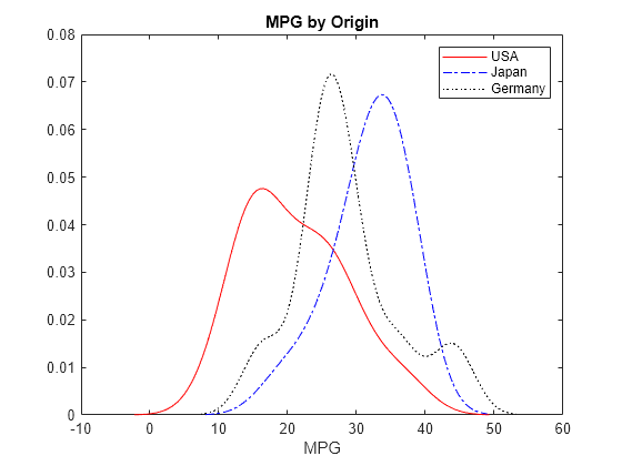
The plot shows how miles per gallon (MPG) performance differs by country of origin (Origin). Using this data, the USA has the widest distribution, and its peak is at the lowest MPG value of the three origins. Japan has the most regular distribution with a slightly heavier left tail, and its peak is at the highest MPG value of the three origins. The peak for Germany is between the USA and Japan, and the second bump near 44 miles per gallon suggests that there might be multiple modes in the data.