fit

Fit incremental normalizer model to streaming data

Since R2026a

Syntax

Normalizer = fit(Normalizer,X)

Normalizer = fit(ClassNormalizer,X,Y)

Normalizer = fit(___,Name=Value)

[Normalizer,XNormalized] = fit(___)

Description

The incremental fit function fits an incremental normalizer model object (ZScoreNormalizer, ExponentiallyWeightedNormalizer, or ClassWeightedNormalizer) to streaming data. The function optionally returns a normalized version of the input data.

Normalizer = fit(Normalizer,X) returns an incremental normalizer model Normalizer (ZScoreNormalizer or ExponentiallyWeidghtedNormalizer model object), which represents the input incremental normalizer model Normalizer fit using the predictor data X. The incremental fit function fits the model to the incoming data and stores the updated normalizer properties in the output model Normalizer.

Normalizer = fit(ClassNormalizer,X,Y) returns an incremental normalizer model Normalizer (ClassWeightedNormalizer model object) which represents the input incremental normalizer model ClassNormalizer fit using the predictor data X and class labels Y.

Normalizer = fit(___,Name=Value) specifies options using one or more name-value arguments in additional to any of the input argument combinations in the previous syntaxes. For example, ObservationsIn="columns" specifies that the columns of X correspond to observations, and the rows correspond to predictors.

[Normalizer,XNormalized] = fit(___) additionally returns the normalized data XNormalized.

Examples

Incremental Normalization

Create a default model for incremental normalization and display its properties.

Normalizer = incrementalNormalizer;
details(Normalizer)

  incremental.preprocessing.ZScoreNormalizer with properties:

               SumOfWeights: [1×0 double]
                  ScaleData: 1
                     Center: [1×0 double]
                      Scale: [1×0 double]
             PredictorNames: []
                     IsWarm: 1
    NumTrainingObservations: 0
              NumPredictors: 0
               WarmupPeriod: 0
             TrainingPeriod: Inf
            UpdateFrequency: 1
      CategoricalPredictors: []

  Methods, Superclasses

Normalizer is a ZScoreNormalizer model object. All its properties are read-only. The properties of Normalizer affect how the incremental fit function processes chunks of data as follows:

• fit returns normalized data (IsWarm=true).

• The ScaleData value is true, meaning that the normalized data is centered (mean = 0) and scaled (standard deviation = 1).

• The UpdateFrequency value is 1, meaning that fit updates the Center (mean) and Scale (standard deviation) values of Normalizer each time it processes an observation.

• The TrainingPeriod value is Inf, meaning that the Center and Scale values of Normalizer are never fixed.

• Because NumPredictors=0, fit sets the NumPredictors value equal to the number of predictors in the input data.

Generate Simulated Data

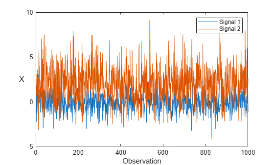
Generate a data set X that contains 1000 observations of two simulated Gaussian noise signals. The first signal has zero mean and a standard deviation of 1, and the second signal has a mean of 2 and a standard deviation of 2.

rng(0,"twister"); % For reproducibility
n = 1000;
X = [randn(n,1),2*randn(n,1)+2];

Plot the data set.

plot(X)
xlabel("Observation")
ylabel("X",Rotation=0)
legend(["Signal 1","Signal 2"])

Perform Incremental Learning

Fit the incremental model Normalizer to the data by using the fit function. To simulate a data stream, fit the model in chunks of 50 observations at a time. At each iteration:

• Process 50 observations.

• Call the incremental fit function to overwrite the previous incremental normalizer model Normalizer with a new one fitted to the incoming observations.

• Store center, the fitted Center values of Normalizer, to see how the values evolve during incremental learning.

• Store scale, the fitted Scale values of Normalizer, to see how the values evolve during incremental learning.

• Store XNormalized, the normalized data chunk, to see how it evolves during incremental learning.

numObsPerChunk = 50;
nchunk = floor(n/numObsPerChunk);
center = zeros(nchunk,2);
scale = zeros(nchunk,2); 
XNormalized = [];
% Incremental normalization
for j = 1:nchunk
    ibegin = min(n,numObsPerChunk*(j-1) + 1);
    iend = min(n,numObsPerChunk*j);
    idx = ibegin:iend;    
    [Normalizer,normalized] = fit(Normalizer,X(idx,:));
    center(j,:) = Normalizer.Center;
    scale(j,:) = Normalizer.Scale;
    XNormalized = [XNormalized;normalized];
end

Display the properties of the incremental normalizer model after the final iteration.

details(Normalizer)

  incremental.preprocessing.ZScoreNormalizer with properties:

               SumOfWeights: [1000 1000]
                  ScaleData: 1
                     Center: [-0.0326 2.0738]
                      Scale: [0.9985 1.9962]
             PredictorNames: ["x1"    "x2"]
                     IsWarm: 1
    NumTrainingObservations: 1000
              NumPredictors: 2
               WarmupPeriod: 0
             TrainingPeriod: Inf
            UpdateFrequency: 1
      CategoricalPredictors: []

  Methods, Superclasses

The model is trained on all the data in the stream. The Center and Scale values are approximately equal to the true means and standard deviations of the input signals.

Analyze Model During Incremental Learning

At the end of each iteration, the fit function updates the Center and Scale values of the model object using the observations in the data chunk. The function then returns a transformed version of the data chunk that is normalized using the updated values of Center and Scale.

To see how the Center and Scale values evolve during training, plot them on separate tiles.

figure
tiledlayout(2,1);
nexttile
plot(center,"o-")
xlabel("Iteration")
ylabel("Center")
nexttile
plot(scale,"o-")
xlabel("Iteration")
ylabel("Scale")

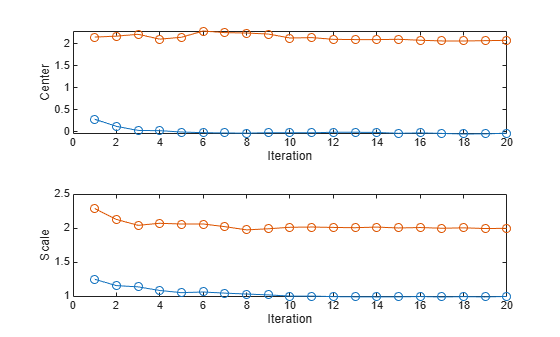
The Center and Scale values approach the true means and standard deviations of the input signals after approximately 10 iterations.

Plot the normalized signal data, and then display the means and standard deviations.

figure
plot(XNormalized)
xlabel("Observation")
ylabel("XNormalized")
legend(["Signal 1","Signal 2"])

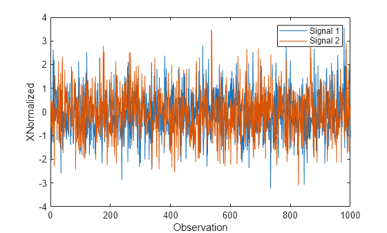
display(mean(XNormalized))

   -0.0323   -0.0318

display(std(XNormalized))

    0.9576    0.9786

The normalized signals have means close to zero and standard deviations close to 1.

Compute the z-scores for the entire data set using the zscore function. Plot the absolute percentage difference between the normalized signal values and the z-scores.

zscores = zscore(X);
figure
plot(100*abs(XNormalized-zscores)/zscores)
xlabel("Observation")
ylabel("Absolute Percentage Difference")
legend(["Signal 1","Signal 2"])

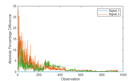
The plot indicates that after the normalizer processes approximately 600 observations, the z-scores and the normalized signal values differ by less than one percent.

Incremental Exponentially Weighted Normalization

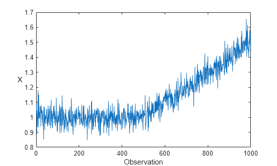
Generate a data set X that contains 1000 observations of a simulated Gaussian noise signal with a standard deviation of 0.05. The signal has an initial mean of 1, which increases linearly after the 500th observation.

rng(0,"twister"); % For reproducibility
n = 1000;
m = 500;
initialMu = 1;
sigma = 0.05;
driftRate = 1/1000;
X = initialMu + sigma*randn(m,1);
t = (1:n-m)';
X = [X; initialMu + t*driftRate + sigma*randn(n-m,1)];

Plot the data set.

plot(X)
xlabel("Observation")
ylabel("X",Rotation=0)

Create Incremental Normalization Model

Create an exponentially weighted incremental normalization model with an initial Center (mean) value of 1 and a Scale (standard deviation) value of 0.05, based on 10 prior observations. Display the properties of the model object.

Normalizer = incrementalNormalizer("exponentiallyweighted", ...
    Center=1,Scale=0.05,NumObservations=10);
details(Normalizer)

  incremental.preprocessing.ExponentiallyWeightedNormalizer with properties:

               SumOfWeights: 10
           ForgettingFactor: 0.0500
                  ScaleData: 1
                     Center: 1
                      Scale: 0.0500
             PredictorNames: "x1"
                     IsWarm: 1
    NumTrainingObservations: 0
              NumPredictors: 1
               WarmupPeriod: 0
             TrainingPeriod: Inf
            UpdateFrequency: 1
      CategoricalPredictors: []

  Methods, Superclasses

Normalizer is an ExponentiallyWeightedNormalizer model object. All its properties are read-only. The properties of Normalizer affect how the software processes chunks of data as follows:

• The incremental fit function returns normalized data (IsWarm=true).

• The ScaleData value is true, meaning that the normalized data is centered (mean = 0) and scaled (standard deviation = 1).

• fit updates the Center and Scale values of the model each time it processes an observation (UpdateFrequency=1).

• The value of ForgettingFactor (0.05) is greater than zero, meaning that fit assigns higher weight to newer observations.

• The TrainingPeriod value is Inf, meaning that the Center and Scale values of the model are never fixed.

Perform Incremental Fitting

To simulate a data stream, process the data in chunks of 50 observations at a time. At each iteration:

• Process 50 observations.

• If the mean of the data chunk is within one standard deviation of the signal's initial mean, transform the data chunk using the current model. Otherwise, overwrite the previous incremental model with a new one fitted to the incoming observations, and then transform the data chunk using the updated values of Center and Scale.

• Store center, the fitted Center value of Normalizer, to see it evolves during incremental learning.

• Store scale, the fitted Scale value of Normalizer, to see how it evolves during incremental learning.

• Store XNormalized, the normalized data chunk, to see how it evolves during incremental learning.

numObsPerChunk = 50;
nchunk = floor(n/numObsPerChunk);
center = zeros(nchunk,1);
scale = zeros(nchunk,1); 
XNormalized = [];
% Incremental normalization
for j = 1:nchunk
    ibegin = min(n,numObsPerChunk*(j-1) + 1);
    iend = min(n,numObsPerChunk*j);
    idx = ibegin:iend;
    chunkMu = mean(X(idx));
    if abs(chunkMu - initialMu) < sigma
        normalized = transform(Normalizer,X(idx));
    else
        [Normalizer,normalized] = fit(Normalizer,X(idx));
    end
    center(j) = Normalizer.Center;
    scale(j) = Normalizer.Scale;
    XNormalized = [XNormalized;normalized];
end

Analyze Incremental Model During Training

To see how the Center and Scale values evolve during training, plot them on separate tiles.

figure
tiledlayout(2,1);
nexttile
plot(center,"o-")
xlabel("Iteration")
ylabel("Center")
nexttile
plot(scale,"o-")
xlabel("Iteration")
ylabel("Scale")

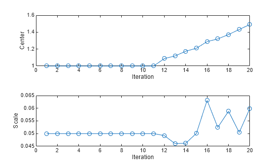
The Center and Scale values closely track the signal's mean and standard deviation values during the first 11 iterations. After the signal's mean starts to drift, the Center value continues to track the signal's mean, and the Scale value fluctuates slightly around the signal's standard deviation value.

Plot the normalized signal data, and then display its mean and standard deviation.

figure
plot(XNormalized)
xlabel("Observation")
ylabel("XNormalized")

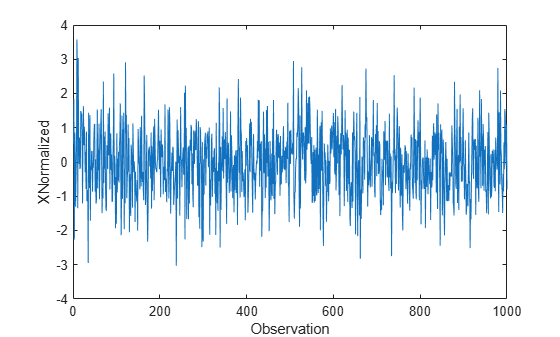
display(mean(XNormalized))

   -0.0180

display(std(XNormalized))

    0.9880

The normalized signal has a mean close to zero and a standard deviation close to 1.

Normalize Data During Incremental Learning

Load the human activity data set. The data set contains 24,075 observations of five physical human activities: sitting, standing, walking, running, and dancing. Each observation has 60 features extracted from acceleration data measured by smartphone accelerometer sensors.

rng(0,"twister") % For reproducibility
load humanactivity
n = numel(actid);
classes = unique(actid);

Display a bar chart of the feature means.

bar(mean(feat))
xlabel("Feature")
ylabel("Mean Value")

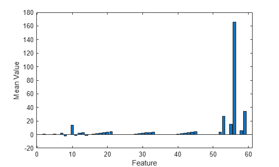
The plot shows that feature 56 has a significantly higher mean than the other features. This result suggests that it is useful to normalize the data prior to incremental learning by converting the data to z-scores, which have a mean of zero and a standard deviation of 1.

Create Incremental Learning Models

For the purposes of this example, perform incremental learning using three methods:

• Normalize the incoming data using simple weighting, and then fit the normalized data using a classification ECOC model that does not perform normalization.

• Normalize the incoming data using class weighting, and then fit the normalized data using a classification ECOC model that does not perform normalization.

• Fit the incoming data using a classification ECOC model that performs normalization.

Create an incremental normalizer model named normalizerSW that uses simple weighting.

normalizerSW = incrementalNormalizer("zscore");

Create an incremental normalizer model named normalizerCW that uses class-weighted normalization. Use the activity class numbers in actid as the class names, and assign prior probabilities based on the frequencies of the activity classes in the data.

frequencies = histcounts(feat, [classes; max(classes) + 1])/n;
normalizerCW = incrementalNormalizer("classweighted",classes,frequencies);

Create two incremental classification ECOC models for multiclass learning. First, configure binary learner properties by creating an incrementalClassificationLinear object. Set the linear classification model type (Learner) to logistic regression, use the sgd solver, and specify to not normalize the input data.

binaryMdl = incrementalClassificationLinear(Learner="logistic", ...
    Standardize=false,Solver="sgd");

Configure the incremental ECOC models as follows:

• Set the maximum number of classes equal to the number of activity states in the data.

• Specify a metrics warm-up period of 5000 observations.

• Specify a metrics window size of 500 observations.

• Specify to use the binary learner binaryMdl for the learners.

mdlSW = incrementalClassificationECOC(MaxNumClasses=length(classes), ...
    MetricsWarmupPeriod=5000,MetricsWindowSize=500,Learners=binaryMdl);
mdlCW = incrementalClassificationECOC(MaxNumClasses=length(classes), ...
    MetricsWarmupPeriod=5000,MetricsWindowSize=500,Learners=binaryMdl);

Create a third incremental ECOC model that normalizes the input data and does not use binaryMdl.

mdl = incrementalClassificationECOC(MaxNumClasses=length(classes), ...
    MetricsWarmupPeriod=5000,MetricsWindowSize=500);

mdlSW, mdlCW, and mdl are incrementalClassificationECOC model objects configured for incremental learning. By default, incrementalClassificationECOC uses classification error loss to measure the performance of the model.

Perform Incremental Fitting

Fit the incremental models to the data by using the fit and updateMetricsAndFit functions. At each iteration:

• Simulate a data stream by processing a chunk of 50 observations.

• Call the updateMetricsAndFit function to overwrite the incremental ECOC model mdl with a new one fitted to the unnormalized data, and to update the performance metrics.

• Call the incremental fit function to overwrite the previous simple-weighted incremental normalizer model NormalizerSW with a new one fitted to the incoming observations. Return the normalized data normalized.

• Store the center (mean) and scale (standard deviation) values of NormalizerSW to see how they evolve during incremental learning.

• Call the updateMetricsAndFit function to overwrite the previous incremental ECOC model mdlSW with a new one fitted to the normalized data, and to update the performance metrics.

• Store the cumulative and window metrics of mdlSW to see how they evolve during incremental learning.

• Repeat the previous four steps using the class-weighted incremental normalizer model NormalizerCW and the incremental ECOC model mdlCW.

During incremental learning, after each model is warmed up, updateMetricsAndFit checks the performance of the model on the incoming observations, and then fits the model to those observations.

% Preallocation
numObsPerChunk = 50;
nchunk = floor(n/numObsPerChunk);
ceSW = array2table(zeros(nchunk,2),VariableNames=["Cumulative","Window"]);
ceCW = array2table(zeros(nchunk,2),VariableNames=["Cumulative","Window"]);
ce = array2table(zeros(nchunk,2),VariableNames=["Cumulative","Window"]);
centerSW = zeros(nchunk,60);
scaleSW = zeros(nchunk,60);
centerCW = zeros(nchunk,60);
scaleCW = zeros(nchunk,60);

% Incremental fitting
for j = 1:nchunk
    ibegin = min(n,numObsPerChunk*(j-1) + 1);
    iend   = min(n,numObsPerChunk*j);
    idx = ibegin:iend; 
    
    mdl = updateMetricsAndFit(mdl,feat(idx,:),actid(idx));
    ce{j,:} = mdl.Metrics{"ClassificationError",:};

    [normalizerSW,normalized] = fit(normalizerSW, feat(idx,:));
    centerSW(j,:) = normalizerSW.Center;
    scaleSW(j,:) = normalizerSW.Scale;
    mdlSW = updateMetricsAndFit(mdlSW,normalized,actid(idx));
    ceSW{j,:} = mdlSW.Metrics{"ClassificationError",:};

    [normalizerCW,normalized] = fit(normalizerCW, feat(idx,:),actid(idx,:));
    centerCW(j,:) = normalizerCW.Center;
    scaleCW(j,:) = normalizerCW.Scale;
    mdlCW = updateMetricsAndFit(mdlCW,normalized,actid(idx));
    ceCW{j,:} = mdlCW.Metrics{"ClassificationError",:};
end

To see how the Center and Scale values of the incremental normalizer models for feature 56 evolve during training, plot them on separate tiles.

figure
t = tiledlayout(2,1);
nexttile
plot([centerSW(:,56) centerCW(:,56)])
ylabel("Center")
xlim([0 nchunk])
legend(["Simple weighted" "Class weighted"],Location="southeast")
nexttile
plot([scaleSW(:,56) scaleCW(:,56)])
ylabel("Scale")
xlim([0 nchunk])
legend(["Simple weighted" "Class weighted"],Location="southeast")
xlabel("Iteration")

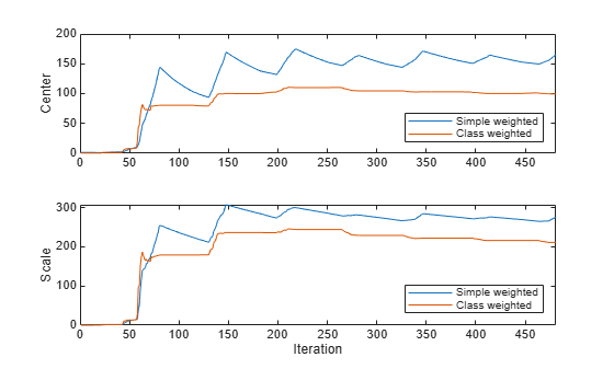
The plots show that the Center and Scale values of feature 56 for both models rise sharply after the 55th iteration, and approach approximately constant values after the 350th iteration. The final values of Center and Scale are different for each model because they use different weighting schemes.

To see how the performance metrics of the incremental ECOC models evolve during training, plot them on separate tiles.

figure
t = tiledlayout(3,1);
nexttile
plot(ceSW.Variables)
ylabel("mdlSW Error")
xlim([0 nchunk])
xline(mdlSW.MetricsWarmupPeriod/numObsPerChunk,"--")
ylim([0 0.25])
legend(ceSW.Properties.VariableNames,Location="northwest")
text(310,0.2,"Simple-weighted normalization",FontSize=8)
nexttile
plot(ceCW.Variables)
xlim([0 nchunk])
ylim([0 0.25])
ylabel("mdlCW Error")
xline(mdlCW.MetricsWarmupPeriod/numObsPerChunk,"--")
legend(ceCW.Properties.VariableNames,Location="northwest")
text(310,0.2,"Class-weighted normalization",FontSize=8)
nexttile
plot(ce.Variables)
xlim([0 nchunk])
ylim([0 0.25])
ylabel("mdl Error")
xline(mdl.MetricsWarmupPeriod/numObsPerChunk,"--")
legend(ce.Properties.VariableNames,Location="northwest")
text(310,0.2,"ECOC model normalization",FontSize=8)
xlabel("Iteration")

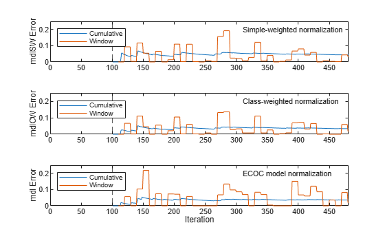
The plots indicate that updateMetricsAndFit performs the following actions:

• Compute the performance metrics after the metrics warm-up period (dashed vertical line at 100th iteration) only.

• Compute the cumulative metrics during each iteration.

• Compute the window metrics after processing 500 observations (10 iterations).

A comparison of the plots indicates that, for this data set, the three incremental learning methods produce similar levels of classification error.

Input Arguments

Normalizer — Incremental normalizer model

ZScoreNormalizer model object | ExponentiallyWeightedNormalizer model object

Incremental normalizer model, specified as a ZScoreNormalizer or ExponentiallyWeightedNormalizer model object. You create Normalizer by calling incrementalNormalizer.

X — Chunk of predictor data

floating-point matrix

Chunk of predictor data, specified as a floating-point matrix of n observations and Normalizer.NumPredictors variables. When ObservationsIn="rows" (the default), the rows of X correspond to observations, and the columns correspond to variables. The incremental fit function ignores observations that contain at least one missing value.

If Normalizer.NumPredictors is 0, fit infers the number of predictors from X, and sets the corresponding property of the output model. Otherwise, if the number of predictor variables in the streaming data changes from Normalizer.NumPredictors, fit issues an error.

Data Types: single | double

ClassNormalizer — Class-weighted incremental normalizer model

ClassWeightedNormalizer model object

Class-weighted incremental normalizer model, specified as a ClassWeightedNormalizer model object. You create ClassNormalizer by calling incrementalNormalizer.

Y — Class labels

categorical array | character array | string array | logical vector | numeric vector | cell array of character vectors

Class labels, specified as a categorical, character, or string array, a logical or numeric vector, or a cell array of character vectors.

• When Normalizer is a ClassWeightedNormalizer object, you must specify Y.

• The length of Y must be equal to the number of observations in X.

• If Y is a character array, then each label must correspond to one row of the array.

• Each element in Y must be a class name in Normalizer.ClassNames. The fit function considers NaN, '' (empty character vector), "" (empty string), <missing>, and <undefined> values in Y to be missing values.

• When processing observations, fit ignores observations that have a missing Y value.

Data Types: single | double | categorical | logical | char | string | cell

Name-Value Arguments

Specify optional pairs of arguments as Name1=Value1,...,NameN=ValueN, where Name is the argument name and Value is the corresponding value. Name-value arguments must appear after other arguments, but the order of the pairs does not matter.

Example: fit(Normalizer,X,ObservationsIn="columns",Weights=W) specifies that the columns of the predictor matrix correspond to observations, and the vector W contains observation weights to apply during incremental learning.

ObservationsIn — Predictor data observation dimension

"rows" (default) | "columns"

Predictor data observation dimension, specified as "rows" or "columns".

Example: ObservationsIn="columns"

Data Types: char | string

Weights — Chunk of observation weights

floating-point vector of positive values

Chunk of observation weights, specified as a floating-point vector of positive values. You cannot specify Weights if Normalizer is an ExponentiallyWeightedNormalizer object. The incremental fit function weighs the observations in X with the corresponding values in Weights. The size of Weights must equal n, the number of observations in X. fit ignores observations that have a Weights value equal to NaN.

By default, Weights is ones(n,1).

Data Types: single | double

Output Arguments

Normalizer — Updated incremental normalizer model

ZScoreNormalizer model object | ExponentiallyWeightedNormalizer model object | ClassWeightedNormalizer model object

Updated incremental normalizer model, returned as a ZScoreNormalizer, ExponentiallyWeightedNormalizer, or ClassWeightedNormalizer model object. When Normalizer.UpdateFrequency is 1 (the default), fit updates Normalizer.Center (and Normalizer.Scale, if Normalizer.ScaleData is true) each time it processes an observation. Otherwise, fit performs the update each time it processes Normalizer.UpdateFrequency observations. When fit processes Normalizer.TrainingPeriod or more observations (Normalizer.NumTrainingObservations ≥ Normalizer.TrainingPeriod), the function does not update Normalizer.Center or Normalizer.Scale.

XNormalized — Normalized data

floating-point matrix

Normalized data, returned as a floating-point matrix. The data type of XNormalized is the same as the data type of X. When ObservationsIn="rows" (the default), the rows of XNormalized correspond to observations, and the columns correspond to variables.

For the noncategorical predictors in the input Normalizer:

• If Normalizer is warm (IsWarm is true), then XNormalized contains z-scores, which the incremental fit function calculates after it processes the last observation in X. Otherwise, all values of XNormalized are NaN. For more information about z-scores, see zscore.

• If Normalizer.ScaleData is true (the default), then fit calculates the XNormalized values using the Normalizer.Center (mean) and Normalizer.Scale (standard deviation) values.

• If Normalizer.ScaleData is false, then fit calculates the XNormalized values using the Normalizer.Center values and a standard deviation of 1.

• If a value in Normalizer.Scale is 0, then all values of the corresponding predictor in XNormalized are 0.

For the categorical predictors specified in Normalizer.CategoricalPredictors, the fit function returns the input data X. However, if Normalizer is not warm (IsWarm is false), all values of XNormalized are NaN.

Algorithms

The fit function normalizes by n–1 when calculating the Scale values, where n is the number of observations in X.

When a value in Normalizer.Scale is 0 or [], the fit function computes the z-score values of the corresponding predictor using a standard deviation value of 1. This behavior matches the behavior of zscore, which computes z-score values using a standard deviation value of 1 when the input data consists of identical values. The normalize function always calculates z-scores using the standard deviation of the input data.

Version History

Introduced in R2026a