Main Content

scaleSpectrum

Scale-averaged wavelet spectrum

Since R2020b

    Description

    example

    savgp = scaleSpectrum(fb,x) returns the scale-averaged wavelet power spectrum of the signal x using the CWT filter bank fb. By default, savgp is obtained by scale-averaging the magnitude-squared scalogram over all scales.

    savgp = scaleSpectrum(fb,cfs) returns the scale-averaged wavelet spectrum for the CWT coefficients cfs.

    Note

    When using this syntax, the power of the scale-averaged wavelet spectrum is normalized to equal the variance of the last signal processed by the filter bank object function wt.

    [savgp,scidx] = scaleSpectrum(___) also returns the scale indices over which the scale-averaged wavelet spectrum is computed. If you do not specify FrequencyLimits or PeriodLimits, scidx is a vector from 1 to the number of scales.

    example

    [___] = scaleSpectrum(___,Name,Value) specifies additional options using name-value pair arguments. These arguments can be added to any of the previous input syntaxes. For example, 'Normalization','none' specifies no normalization of the scale-averaged wavelet spectrum.

    scaleSpectrum(___) with no output arguments plots the scale-averaged wavelet power spectrum in the current figure.

    Examples

    collapse all

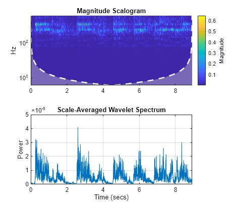
    Load an audio file containing a fragment of Handel's "Hallelujah Chorus" sampled at 8192 Hz.

    load handel         % To hear, type soundsc(y,Fs)

    Create a CWT filter bank that can be applied to the signal. Use the default Morse wavelet.

    fb = cwtfilterbank('SignalLength',length(y),'SamplingFrequency',Fs);

    Plot the scalogram and scale-averaged wavelet power spectrum using the default settings.

    scaleSpectrum(fb,y)

    Figure contains 2 axes objects. Axes object 1 with title Magnitude Scalogram, ylabel Hz contains 3 objects of type image, line, area. Axes object 2 with title Scale-Averaged Wavelet Spectrum, xlabel Time (secs), ylabel Power contains an object of type line.

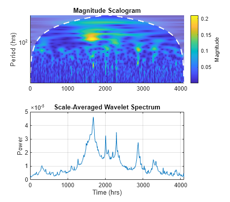
    Load a time series of solar magnetic field magnitudes recorded hourly over the south pole of the sun by the Ulysses spacecraft from 21:00 UT on December 4, 1993 to 12:00 UT on May 24, 1994. See [2] pp. 218–220 for a complete description of this data. Create a CWT filter bank that can be applied to the data. Plot the scalogram and the scale-averaged wavelet spectrum.

    load solarMFmagnitudes
    fb = cwtfilterbank('SignalLength',length(sm),'SamplingPeriod',hours(1));
    scaleSpectrum(fb,sm)

    Figure contains 2 axes objects. Axes object 1 with title Magnitude Scalogram, ylabel Period (hrs) contains 3 objects of type image, line, area. Axes object 2 with title Scale-Averaged Wavelet Spectrum, xlabel Time (hrs), ylabel Power contains an object of type line.

    Obtain the scale-averaged wavelet spectrum of the signal using default values. By default, scaleSpectrum normalizes the power of the scale-averaged wavelet spectrum to equal the variance of the signal. Verify that the sum of the spectrum equals the variance of the signal.

    savg = scaleSpectrum(fb,sm);
    [var(sm) sum(savg)]
    ans = 1×2
    
        0.0448    0.0447


    Obtain the scale-averaged wavelet spectrum of the signal, but instead normalize the power as a probability density function. Verify that the sum is equal to 1.

    savg = scaleSpectrum(fb,sm,'Normalization','pdf');
    sum(savg)
    ans = 1.0000
    

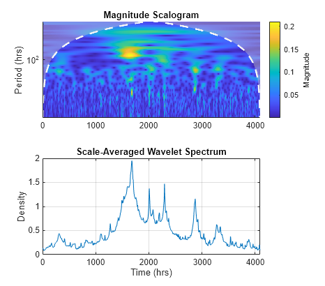
    If you set SpectrumType to 'density', scaleSpectrum normalizes the weighted integral of the wavelet spectrum according to the value of Normalization. In this case, the spectrum mimics a probability density function whose integral, numerically evaluated, equals the value specified by Normalization.

    Plot the scalogram and the scale-averaged wavelet spectrum with spectrum type 'density' and 'pdf' normalization.

    figure
    scaleSpectrum(fb,sm,'SpectrumType','density','Normalization','pdf')

    Figure contains 2 axes objects. Axes object 1 with title Magnitude Scalogram, ylabel Period (hrs) contains 3 objects of type image, line, area. Axes object 2 with title Scale-Averaged Wavelet Spectrum, xlabel Time (hrs), ylabel Density contains an object of type line.

    To confirm the integral of the spectrum equals 1, first obtain the scale-averaged wavelet spectrum with 'density' spectrum type and 'pdf' normalization.

    savg = scaleSpectrum(fb,sm,'SpectrumType','density','Normalization','pdf');

    By default, the filter bank uses the analytic Morse (3,60) wavelet. Obtain the admissibility constant for the wavelet and numerically integrate the wavelet spectrum using the trapezoidal rule. Confirm that the integral equals 1.

    ga = 3;
    tbw = 60;
    
    be = tbw/ga;
    anorm = 2*exp(be/ga*(1+(log(ga)-log(be))));
    cPsi = anorm^2/(2*ga).*(1/2)^(2*(be/ga)-1)*gamma(2*be/ga);
    
    numInt = 2/cPsi*1/length(sm)*trapz(1:length(savg),savg)
    numInt = 1.0000
    

    Input Arguments

    collapse all

    Continuous wavelet transform (CWT) filter bank, specified as a cwtfilterbank object.

    Input data, specified as a real- or complex-valued vector. The input data x must have at least four samples.

    Data Types: single | double
    Complex Number Support: Yes

    CWT coefficients, specified as a 2-D matrix or as an M-by-N-by-2 array. cfs should be the output of the wt object function of the CWT filter bank fb.

    Data Types: single | double
    Complex Number Support: Yes

    Name-Value Arguments

    Specify optional pairs of arguments as Name1=Value1,...,NameN=ValueN, where Name is the argument name and Value is the corresponding value. Name-value arguments must appear after other arguments, but the order of the pairs does not matter.

    Before R2021a, use commas to separate each name and value, and enclose Name in quotes.

    Example: scaleSpectrum(fb,x,'FrequencyLimits',[0.2 0.4]) returns the scale-averaged wavelet spectrum averaged over the frequency limits [0.2 0.4].

    Normalization of the scale-averaged wavelet spectrum, specified as a comma-separated pair consisting of 'Normalization' and one of the following:

    • 'var' — Normalize to equal the variance of the time series x. If you provide the cfs input, the scaleSpectrum function uses the variance of the last time series processed by the filter bank object function wt.

    • 'pdf' — Normalize to equal 1.

    • 'none' — No normalization is applied.

    Type of wavelet spectrum to return, specified as a comma-separated pair consisting of 'SpectrumType' and either 'power' or 'density'. If specified as 'power', the averaged sum of the scale-averaged wavelet spectrum over all scales is normalized according to the value specified in 'Normalization'. If specified as 'density', the weighted integral of the wavelet spectrum over all scales is normalized according to the value specified in 'Normalization'.

    Frequency limits over which the magnitude-squared scalogram is averaged, specified as a comma-separated pair consisting of 'FrequencyLimits' and a two-element vector with nondecreasing elements. The FrequencyLimits values must lie between the lowest and highest center frequencies returned by the centerFrequencies object function of fb. The base 2 logarithm of the ratio of the maximum frequency to the minimum frequency must be greater than or equal to 1/NV, where NV is the value of the 'VoicesPerOctave' property of the filter bank fb.

    If a region of the specified limits falls outside the frequency limits of the filter bank fb, scaleSpectrum truncates computations to within the range specified by centerFrequencies(fb). FrequencyLimits cannot be completely outside of the Nyquist range.

    Period limits over which the magnitude-squared scalogram is averaged, specified as a comma-separated pair consisting of 'PeriodsLimits' and a two-element vector with nondecreasing durations. The elements of PeriodLimits agree in type and format with the 'SamplingPeriod' property of the filter bank fb. The SamplingPeriod values must lie between the lowest and highest center periods returned by the centerPeriods object function of fb. The base 2 logarithm of the ratio of the minimum period to the maximum period must be less than or equal to -1/NV, where NV is the value of the 'VoicesPerOctave' property of the filter bank fb.

    If a region of the specified limits falls outside the period limits of the filter bank fb, scaleSpectrum truncates computations to within the range specified by centerPeriods(fb). SamplingPeriod cannot be completely outside the Nyquist range of [2*Ts,N*Ts], where Ts is the 'SamplingPeriod' and N is the signal length.

    Output Arguments

    collapse all

    Scale-averaged wavelet power spectrum, returned as a real-valued vector or real-valued 3-D array. If x is real-valued, savgp is a 1-by-N vector where N is the length of x. If x is complex-valued, savgp is a 1-by-N-by-2 array, where the first page is the scale-averaged wavelet spectrum for the positive scales (analytic part or counterclockwise component), and the second page is the scale-averaged wavelet spectrum for the negative scales (anti-analytic part or clockwise component).

    Scale indices over which the scale-average wavelet spectrum is computed, returned as a vector. If you do not specify 'FrequencyLimits' or 'PeriodLimits', scidx is a vector from 1 to the number of scales.

    References

    [1] Torrence, Christopher, and Gilbert P. Compo. “A Practical Guide to Wavelet Analysis.” Bulletin of the American Meteorological Society 79, no. 1 (January 1, 1998): 61–78. https://doi.org/10.1175/1520-0477(1998)079<0061:APGTWA>2.0.CO;2.

    [2] Percival, Donald B., and Andrew T. Walden. Wavelet Methods for Time Series Analysis. Cambridge Series in Statistical and Probabilistic Mathematics. Cambridge ; New York: Cambridge University Press, 2000.

    [3] Lilly, J.M., and S.C. Olhede. “Higher-Order Properties of Analytic Wavelets.” IEEE Transactions on Signal Processing 57, no. 1 (January 2009): 146–60. https://doi.org/10.1109/TSP.2008.2007607.

    Extended Capabilities

    Version History

    Introduced in R2020b