Main Content

timeSpectrum

Time-averaged wavelet spectrum

Since R2020b

    Description

    tavgp = timeSpectrum(fb,x) returns the time-averaged wavelet power spectrum of the signal x using the continuous wavelet transform (CWT) filter bank fb. By default, tavgp is obtained by time-averaging the magnitude-squared scalogram over all times. The power of the time-averaged wavelet spectrum is normalized to equal the variance of x.

    tavgp = timeSpectrum(fb,cfs) returns the time-averaged wavelet spectrum for the CWT coefficients cfs.

    Note

    When using this syntax, the power of the time-averaged wavelet spectrum is normalized to equal the variance of the last signal processed by the filter bank object function wt.

    example

    [tavgp,f] = timeSpectrum(___) returns the wavelet center frequencies or center periods for the time-averaged wavelet spectrum. f is a column vector or duration array depending on whether the sampling frequency or sampling period is specified in the CWT filter bank, fb.

    example

    [___] = timeSpectrum(___,Name,Value) specifies additional options using name-value pair arguments. These arguments can be added to any of the previous input syntaxes. For example, 'Normalization','none' specifies no normalization of the time-averaged wavelet spectrum.

    timeSpectrum(___) with no output arguments plots the time-averaged wavelet power spectrum in the current figure.

    Examples

    collapse all

    Load the NPG2006 dataset [1]. The data is the trajectory of a subsurface float trapped in an eddy. Plot the eastward and northward displacement. The triangle marks the initial position.

    load npg2006
    plot(npg2006.cx)
    hold on
    grid on
    xlabel('Eastward Displacement (km)')
    ylabel('Northward Displacement (km)')
    plot(npg2006.cx(1),'^','markersize',11,'color','r',...
        'markerfacecolor',[1 0 0 ])

    Figure contains an axes object. The axes object with xlabel Eastward Displacement (km), ylabel Northward Displacement (km) contains 2 objects of type line. One or more of the lines displays its values using only markers

    Create a CWT filter bank that can be applied to the data. Use the default Morse wavelet. The sampling period for the data is 4 hours.

    fb = cwtfilterbank('SignalLength',length(npg2006.cx),'SamplingPeriod',hours(4));

    Obtain the time-averaged wavelet power spectra and the center periods.

    [tavgp,centerP] = timeSpectrum(fb,npg2006.cx);
    size(tavgp)
    ans = 1×3
    
        73     1     2


    The first page is the time-averaged wavelet spectrum for the positive scales (analytic part or counterclockwise component), and the second page is the time-averaged wavelet spectrum for the negative scales (anti-analytic part or clockwise component). Plot both spectra.

    subplot(2,1,1)
    plot(centerP,tavgp(:,1,1))
    title('Counterclockwise Component')
    ylabel('Power')
    xlabel('Period (hrs)')
    subplot(2,1,2)
    plot(centerP,tavgp(:,1,2))
    title('Clockwise Component')
    ylabel('Power')
    xlabel('Period (hrs)')

    Figure contains 2 axes objects. Axes object 1 with title Counterclockwise Component, xlabel Period (hrs), ylabel Power contains an object of type line. Axes object 2 with title Clockwise Component, xlabel Period (hrs), ylabel Power contains an object of type line.

    If you omit the output arguments and execute timeSpectrum(fb,npg2006.cx) on the command line, the scalograms and time-averaged power spectra are plotted in the current figure. Note that the clockwise rotation of the float is captured in the clockwise rotary scalogram and the time-averaged spectrum.

    2020-07-11_17-05-16.png

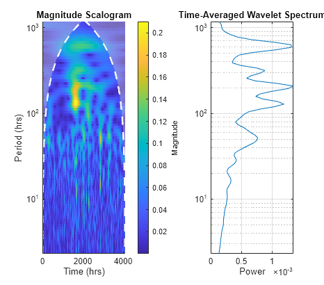
    Load a time series of solar magnetic field magnitudes recorded hourly over the south pole of the sun by the Ulysses spacecraft from 21:00 UT on December 4, 1993 to 12:00 UT on May 24, 1994. See [3] pp. 218–220 for a complete description of this data. Create a CWT filter bank that can be applied to the data. Plot the scalogram and the time-averaged wavelet spectrum.

    load solarMFmagnitudes
    fb = cwtfilterbank('SignalLength',length(sm),'SamplingPeriod',hours(1));
    timeSpectrum(fb,sm)

    Figure contains 2 axes objects. Axes object 1 with title Magnitude Scalogram, xlabel Time (hrs), ylabel Period (hrs) contains 3 objects of type image, line, area. Axes object 2 with title Time-Averaged Wavelet Spectrum, xlabel Power contains an object of type line.

    Obtain the time-averaged wavelet spectrum of the signal using default values. By default, timeSpectrum normalizes the power of the time-averaged wavelet spectrum to equal the variance of the signal. Verify that the sum of the spectrum equals the variance of the signal.

    tavg = timeSpectrum(fb,sm);
    [var(sm) sum(tavg)]
    ans = 1×2
    
        0.0448    0.0447


    Obtain the time-averaged wavelet spectrum of the signal, but instead normalize the power as a probability density function. Verify that the sum is equal to 1.

    tavg = timeSpectrum(fb,sm,'Normalization','pdf');
    sum(tavg)
    ans = 1.0000
    

    If you set SpectrumType to 'density', timeSpectrum normalizes the weighted integral of the wavelet spectrum according to the value of Normalization. The spectrum mimics a probability density function whose integral, numerically evaluated, equals the value specified by Normalization.

    Plot the scalogram and the time-averaged wavelet spectrum with spectrum type 'density' and 'pdf' normalization.

    figure
    timeSpectrum(fb,sm,'SpectrumType','density','Normalization','pdf')

    Figure contains 2 axes objects. Axes object 1 with title Magnitude Scalogram, xlabel Time (hrs), ylabel Period (hrs) contains 3 objects of type image, line, area. Axes object 2 with title Time-Averaged Wavelet Spectrum, xlabel Density contains an object of type line.

    To confirm the integral of the spectrum equals 1, first obtain the time-averaged wavelet spectrum with 'density' spectrum type and 'pdf' normalization.

    tavg = timeSpectrum(fb,sm,'SpectrumType','density','Normalization','pdf');

    By default, the filter bank uses the analytic Morse (3,60) wavelet. Obtain the admissibility constant for the wavelet and numerically integrate the wavelet spectrum using the trapezoidal rule. Keep in mind that the CWT uses L1 normalization. Confirm that the integral equals 1.

    ga = 3;
    tbw = 60;
    
    be = tbw/ga;
    anorm = 2*exp(be/ga*(1+(log(ga)-log(be))));
    cPsi = anorm^2/(2*ga).*(1/2)^(2*(be/ga)-1)*gamma(2*be/ga);
    
    rawScales = scales(fb);
    numInt = 2/cPsi*1/length(sm)*trapz(rawScales(:),tavg./rawScales(:))
    numInt = 1.0000
    

    Input Arguments

    collapse all

    Continuous wavelet transform (CWT) filter bank, specified as a cwtfilterbank object.

    Input data, specified as a real- or complex-valued vector. The input data x must have at least four samples.

    Data Types: single | double
    Complex Number Support: Yes

    CWT coefficients, specified as a 2-D matrix or as an M-by-N-by-2 array. cfs should be the output of the wt object function of the CWT filter bank fb.

    Data Types: single | double
    Complex Number Support: Yes

    Name-Value Arguments

    Specify optional pairs of arguments as Name1=Value1,...,NameN=ValueN, where Name is the argument name and Value is the corresponding value. Name-value arguments must appear after other arguments, but the order of the pairs does not matter.

    Before R2021a, use commas to separate each name and value, and enclose Name in quotes.

    Example: timeSpectrum(fb,x,'TimeLimits',[100 500],'Normalization','none') returns the time-averaged wavelet spectrum averaged over the time limits specified in samples without normalizing the spectrum.

    Normalization of the time-averaged wavelet spectrum, specified as a comma-separated pair consisting of 'Normalization' and one of the following:

    • 'var' — Normalize to equal the variance of the time series x. If you provide the cfs input, the timeSpectrum function uses the variance of the last time series processed by the filter bank object function wt.

    • 'pdf' — Normalize to equal 1.

    • 'none' — No normalization is applied.

    Type of wavelet spectrum to return, specified as a comma-separated pair consisting of 'SpectrumType' and either 'power' or 'density'. If specified as 'power', the averaged sum of the time-averaged wavelet spectrum over all times is normalized according to the value specified in 'Normalization'. If specified as 'density', the weighted integral of the wavelet spectrum over all times is normalized according to the value specified in 'Normalization'.

    Note

    With regards to the numerical implementation of the continuous wavelet transform, the integral over scale is performed using L1 normalization. With L1 normalization, if you have equal amplitude oscillatory components in your data at different scales, they will have equal magnitude in the CWT. Using L1 normalization provides a more accurate representation of the signal. For more information, see L1 Norm for CWT.

    Time limits over which to average the wavelet spectrum, specified in samples. TimeLimits is specified as a comma-separated pair consisting of 'TimeLimits' and a two-element vector with nondecreasing elements. When you specify the input data as a signal, the elements are between 1 and the length of x. When you specify the input data as CWT coefficients, the elements are between 1 and size(cfs,2).

    Output Arguments

    collapse all

    Time-averaged wavelet power spectrum, returned as a real-valued vector or real-valued 3-D array. If x is real-valued, tavgp is an F-by-1 vector, where F is the number of wavelet center frequencies or center periods in the CWT filter bank fb. If x is complex-valued, tavgp is an F-by-1-by-2 array, where the first page is the time-averaged wavelet spectrum for the positive scales (analytic part or counterclockwise component), and the second page is the time-averaged wavelet spectrum for the negative scales (anti-analytic part or clockwise component).

    Center frequencies or center periods for the time-averaged wavelet spectrum, returned as a column vector or duration array, respectively. If the sampling frequency is specified in fb, then the elements of f are the center frequencies ordered from high to low. If the sampling period is specified in fb, then the elements of f are the center periods.

    References

    [1] Lilly, J. M., and J.-C. Gascard. “Wavelet Ridge Diagnosis of Time-Varying Elliptical Signals with Application to an Oceanic Eddy.” Nonlinear Processes in Geophysics 13, no. 5 (September 14, 2006): 467–83. https://doi.org/10.5194/npg-13-467-2006.

    [2] Torrence, Christopher, and Gilbert P. Compo. “A Practical Guide to Wavelet Analysis.” Bulletin of the American Meteorological Society 79, no. 1 (January 1, 1998): 61–78. https://doi.org/10.1175/1520-0477(1998)079<0061:APGTWA>2.0.CO;2.

    [3] Percival, Donald B., and Andrew T. Walden. Wavelet Methods for Time Series Analysis. Cambridge Series in Statistical and Probabilistic Mathematics. Cambridge ; New York: Cambridge University Press, 2000.

    [4] Lilly, J.M., and S.C. Olhede. “Higher-Order Properties of Analytic Wavelets.” IEEE Transactions on Signal Processing 57, no. 1 (January 2009): 146–60. https://doi.org/10.1109/TSP.2008.2007607.

    Extended Capabilities

    C/C++ Code Generation
    Generate C and C++ code using MATLAB® Coder™.

    Version History

    Introduced in R2020b