tffilt

Time-frequency filtering using binary mask and Gabor transform

Since R2025a

Syntax

y = tffilt(bmask,x)

y = tffilt(bmask,x,Name=Value)

Description

y = tffilt(bmask,x) reconstructs the filtered signal y by applying the time-frequency binary mask bmask to the discrete Gabor transform (DGT) of x and inverting the result.

y = tffilt(bmask,x,Name=Value) specifies options using or more name-value arguments, in addition to the input arguments of the previous syntax. For example, to specify a hop length of 16 samples, set HopLength to 16.

Examples

Perform Time-Frequency Filtering of Signal Using Discrete Gabor Transform

Create a signal that consists of a quadratic chirp and two sinusoids whose frequencies are 250 Hz and 350 Hz, respectively. The sinusoids have disjoint time support. Sample the signal at 1 kHz for four seconds.

tspan = 4;
Fs = 1e3;
t = 0:1/Fs:tspan-1/Fs;
chp = chirp(tspan/2-t,30,max(tspan/2-t),100,"quadratic",[],"concave");
si1 = cos(250*2*pi*t);
si2 = cos(350*2*pi*t);
si1 = si1.*(t<tspan/2);
si2 = si2.*(t>=tspan/2);
sig = si1+si2+chp;

Visualize the one-sided discrete Gabor transform of the signal.

dgt(sig,SampleRate=Fs,FrequencyRange="onesided")

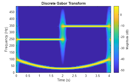
Obtain the DGT of the signal. Also obtain the frequencies and times at which the DGT is evaluated.

[d,frq,tm] = dgt(sig,SampleRate=Fs,FrequencyRange="onesided");

Use the frequency vector and time vector to create time-frequency masks that mark for removal:

• The 250 Hz sinusoid.

• The chirp samples from two to four seconds.

frqSinusoid = (frq>225)&(frq<275);
tmSinusoid = (tm<2);
mskSinusoid = frqSinusoid*tmSinusoid';

frqChirp = (frq<125);
tmChirp = (tm>2);
mskChirp = frqChirp*tmChirp';

Use the tffilt function to reconstruct a filtered signal using the two masks. Specify the "gm" time-frequency filtering method.

rec = tffilt({mskSinusoid,mskChirp},sig,FrequencyRange="onesided", ...
    Method="gm");

Plot the original signal and reconstruction.

tiledlayout(2,1)
nexttile
plot(t,sig)
ylim([-2.2 2.2])
ylabel("Amplitude")
title("Original Signal")
nexttile
plot(t,rec)
ylim([-2.2 2.2])
ylabel("Amplitude")
xlabel("Time (s)")
title("Filtered Signal")

Visualize the DGT of the filtered signal.

figure
dgt(rec,SampleRate=Fs,FrequencyRange="onesided")

Remove Percussive Audio Interference From Mixed Signal

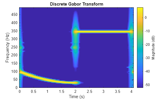
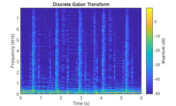
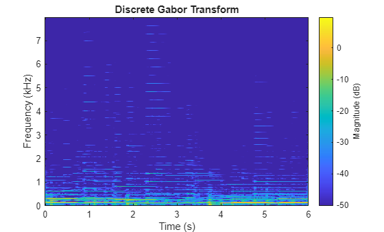
Load the harmperc data file. After loading, your workspace contains the following variables:

• x — A mixed audio recording of a drum and guitar.

• harm — An audio recording of only the guitar.

• fs — A scalar containing the sample rate.

The duration of both recordings is six seconds. The sample rate is 16 kHz.

load harmperc

Use dgt to visualize the one-sided DGT of the mixed recording. Specify a window length of 1024 samples, a hop length of 512 samples. Set the number of frequency bins to $$2^{11}$$.

winLen = 1024;
hopLen = 512;
numBins = 2^11;
dgt(x,WindowLength=winLen,HopLength=hopLen, ...
    SampleRate=fs, ...
    NumFrequencyBins=numBins, ...
    FrequencyRange="onesided")

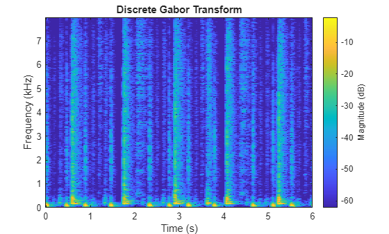
The difference between the mixed and guitar recordings is the percussive audio. Visualize the one-sided DGT of the difference between the two recordings. Use the same dgt parameters.

dgt(x-harm,WindowLength=winLen,HopLength=hopLen, ...
    SampleRate=fs, ...
    NumFrequencyBins=numBins, ...
    FrequencyRange="onesided")

Obtain the DGT of the difference between the two recordings and the mixed recording.

Dp = dgt(x-harm,WindowLength=winLen,HopLength=hopLen, ...
    SampleRate=fs, ...
    NumFrequencyBins=numBins, ...
    FrequencyRange="onesided");
Dx = dgt(x,WindowLength=winLen,HopLength=hopLen, ...
    SampleRate=fs, ...
    NumFrequencyBins=numBins, ...
    FrequencyRange="onesided");

Use both DGTs to create a binary mask that identifies the time-frequency bins associated with the percussive audio to filter out of the DGT of the mixed recording. Keep in mind that a true value indicates that tffilt filters out the corresponding time-frequency bin.

bmask = abs(Dp)>0.5*abs(Dx);

Use tffilt to apply the mask to the mixed audio recording. Use the "gm" time-frequency filtering method. Visualize the DGT of the reconstruction.

y = tffilt(bmask,x,WindowLength=winLen,HopLength=hopLen, ...
    NumFrequencyBins=numBins,FrequencyRange="onesided",Method="gm");
dgt(y,WindowLength=winLen,HopLength=hopLen, ...
    SampleRate=fs, ...
    NumFrequencyBins=numBins,FrequencyRange="onesided");

Compute the signal-to-interference (SIR) before and after the filtering.

sirBefore = 20*log10(norm(harm,2)/norm(harm-x,2))

sirBefore = 
10.4058

sirAfter = 20*log10(norm(harm,2)/norm(harm-y,2))

sirAfter = 
17.2166

Input Arguments

bmask — Binary mask

logical matrix | cell array of logical matrices

Binary mask, specified as a logical matrix or a cell array of logical matrices. The size of each logical matrix must be the same as the size of the DGT of the input signal x. The row and column dimensions correspond to the frequency and time axes, respectively, of the time-frequency plane. A true value indicates that tffilt filters out the corresponding time-frequency bin.

To make the size of the DGT the same as that of bmask, HopLength, NumFrequencyBins, and FrequencyRange must be the same as those used in computing bmask.

If bmask is a cell array, the tffilt function applies each mask sequentially to the DGT of x before reconstructing the filtered signal.

Data Types: logical

x — Input signal

vector | timetable

Input signal, specified as a vector or a timetable with a single variable containing a vector. If x is a timetable, it must contain finite and uniformly increasing row times.

To obtain the DGT of the input signal, x, the tffilt function internally uses the dgt function. If the signal length is not an integer multiple of the least common multiple (LCM) of the hop length, HopLength, and the length of the Gaussian window, WindowLength, dgt zero-pads the signal to the nearest largest length that is a multiple of this LCM.

Data Types: single | double
Complex Number Support: Yes

Name-Value Arguments

Specify optional pairs of arguments as Name1=Value1,...,NameN=ValueN, where Name is the argument name and Value is the corresponding value. Name-value arguments must appear after other arguments, but the order of the pairs does not matter.

Example: y=tffilt(bmask,x,FrequencyRange="onesided",HopLength=32) computes a one-sided DGT using a hop length of 32 samples.

WindowLength — Gaussian window length

128 (default) | positive integer

Gaussian window length in samples, specified as a positive integer. The window length also determines the time-frequency ratio (TFR) of the window. For more information, see Time-Frequency Ratio.

Data Types: single | double

HopLength — Hop length

32 (default) | nonnegative integer

Hop length or time shift of the Gaussian windows in samples, specified as a nonnegative integer. The hop length affects the overlap between the windows and thus the time resolution of the transform.

You must specify the same hop length to create the binary mask bmask.

Data Types: single | double

NumFrequencyBins — Number of frequency bins

256 (default) | positive integer

Number of frequency bins to use to calculate the DGT, specified as a positive integer. The number of bins determines the frequency resolution in the time-frequency representation of the signal.

To ensure the transform is redundant and perfect reconstruction can be achieved, the number of frequency bins must be larger than the hop length.

You must specify the same number of frequency bins to create the binary mask bmask.

Data Types: single | double

FrequencyRange — DGT frequency range

"centered" (default) | "onesided" | "twosided"

DGT frequency range, specified as "centered", "onesided", or "twosided". The tffilt function computes the DGT over the specified range.

• "centered" — Computes a two-sided and centered DGT.

• "onesided" — Computes a one-sided DGT.

• "twosided" — Computes a two-sided DGT.

You must use the same number of frequency bins and frequency range to create the binary mask bmask.

Method — Time-frequency filtering method

"igm" (default) | "gm" | "rigm"

Time-frequency filtering method, specified as one of these:

• "igm" — tffilt performs filtering by reconstructing the signal using the inverse of the Gabor multiplier. This method involves solving a linear system where the Gabor multiplier's eigenvalues are estimated using the iterative preconditioned conjugate gradient technique, allowing effective reconstruction of the filtered signal. tffilt internally uses the pcg and eigs functions.

• "gm" — tffilt performs filtering by applying the binary mask bmask directly to the DGT of the input signal x, and then reconstructing the signal using the inverse DGT. Specifically, the algorithm calculates the filtered signal as IDGT(bmask.*dgt(x)). This method is computationally less intensive compared to the other methods.

• "rigm" — tffilt performs filtering by solving a regularized optimization problem [1]. The function computes the eigenvalues of the Gabor multiplier using the adaptive randomized range finder (ARRF) techniques and the Nystrom method for random eigenvalue decomposition. To learn more about the ARRF and Nystrom algorithms, as implemented in tffilt, see Algorithms 4.2 and 5.5, respectively, in [4].

For more information, see Gabor Multipliers.

Output Arguments

y — Filtered signal

vector | timetable

Filtered signal, returned as a vector or timetable. y has the same size and data type as the input signal x.

More About

Time-Frequency Ratio

The time-frequency ratio (TFR) is the ratio between the effective support of the Gaussian window in time and in frequency. The TFR is computed as $$\pi W^2/4L\log 2$$, where W is the length of the Gaussian window in samples and L is the length of the input signal. The periodic Gaussian is given by

$$g_p={\displaystyle \sum _{p=-P}^{P}g}(l-pL),$$

where $$g(l)=\exp \left(-\pi \frac{l^2}{L\text{TFR}}\right),l=0,\dots ,L-1$$ and $$P=\lceil 4/\sqrt{\raisebox{1ex}{$L$}\!\left/ \!\raisebox{-1ex}{$\sqrt{\text{TFR}}$}\right.}\rceil$$ [2].

If the TFR is greater than 1, then the window has a wider support in the time domain.

Gabor Frames

A set of functions $$\left\{g_{m,n}(l)=g(l-an)e^{2\pi ılm/M}\right\}$$ forms a Gabor frame if there exist positive constants A and B such that:

$$A\Vert x{\Vert }^2\le {\displaystyle \sum _{m,n}|\langle x,g_{m,n}\rangle {|}^2}\le B\Vert x{\Vert }^2$$

for all signals x, where A and B are frame bounds. This condition ensures that the signal can be accurately represented and reconstructed.

When A = B = 1, the frame is called a Parseval Gabor frame. For more information, see Nonstationary Gabor Frames and the Constant-Q Transform.

Discrete Gabor Transform

The discrete Gabor transform (DGT) is a commonly used transform in signal analysis and synthesis, especially when a linear frequency scale is required. The DGT of a discrete signal is computed based on the canonical tight window of a Gabor frame with a periodic Gaussian window [3]. The DGT is computed by sliding the Gaussian window over the signal and calculating the DGT of each segment of windowed data.

The DGT of a discrete signal x is given as:

$$D(m,n)={\displaystyle \sum _{l=0}^{L-1}x}(l)\overline{g(l-an)}{e}^{-2\pi ılm/M},$$

where:

• g(l) is the (analysis) window function (filter prototype) that localizes the signal in time and in frequency. The bar over the window function indicates complex conjugate.

• a is the hop length, which determines how much the window is shifted for each time step.

• M is the number of frequency points (frequency bins), determining the frequency resolution.

• L is the signal length that satisfies L = a N = b M, where N and b are positive integers.

• D(m,n) are the time-frequency coefficients, representing the signal's content at time index n and frequency index m.

By default, the tffilt function shifts the Gaussian window, whose length is 128 samples, by 32 samples in time. This yields an overlap of 75%.

Inverse Discrete Gabor Transform

The inverse discrete Gabor transform (IDGT) reconstructs the original signal x from the DGT coefficients.

Using the notation from above, the IDGT is given as:

$$V^H\text{D}(l)=\sum _{n=0}^{N-1}\sum _{m=0}^{M-1}\text{D}(m,n)\gamma (l-an)e^{2\pi ıml/M}=\underset{}{\overset{ˆ}{x}}(l)$$

where $$\gamma (l)$$ is the synthesis window function. To ensure perfect reconstruction, the following must be satisfied:

• Frame Condition — The sets of analysis window functions, $$\{g_{m,n}(l)\}=\{g(l-an)e^{2\pi ıml/M}\}$$, and synthesis window functions, $$\{{\gamma }_{m,n}(l)\}=\{\gamma (l-an)e^{2\pi ıml/M}\}$$, must each form a Parseval Gabor frame.

• Redundancy — The redundancy factor $$R$$ of a Gabor frame $$G(g,a,M)$$ is defined as $$\rho =M/a$$. For perfect reconstruction, $$\rho \ge 1$$.

Gabor Multipliers

Gabor multipliers are linear operators used for time-varying signal filtering through pointwise multiplication in the Gabor domain.

Defined by a window function $$g$$, an integer lattice $$\Lambda =(a,M)$$, and $$M$$-by-$$N$$mask $$\text{m}$$, a Gabor multiplier (GM) $$M$$ acts on a signal $$x$$ as:

$$M_{m}x=V^{H}mVx=\sum _{m=0}^{M-1}\sum _{n=0}^{N-1}m(m,n)⟨x,g_{m,n}⟩{\gamma }_{m,n}.$$

The tffilt function uses three methods to perform filtering.

• "gm" — The function returns the output of the GM.

• "igm" — The function uses an iterative approach based on the precondition conjugate gradient algorithm to find the inverse of the GM.

• "rigm" — The function solves the optimization problem $${\underset{}{\overset{ˆ}{x}}}_{\lambda }^{(d)}=\arg \underset{z}{\min }{\Vert Vz-Vx\Vert }_{\underset{}{\overset{‾}{\Omega }}}^2+\sum _{p=1}^P{\lambda }_p{\Vert Vz\Vert }_{{\Omega }_p}^2$$, where $${\Omega }_p$$ is the subregion in the time-frequency domain $$\Lambda$$, $${\lambda }_p>0$$ is a regularizing factor, and $$x=x^{(d)}+\text{interference}$$ is the observed signal and $$x^{(d)}$$ is the desired signal to be reconstructed. The region $$\Omega =\bigcup _p{\Omega }_p=\Lambda \backslash \underset{}{\overset{‾}{\Omega }}$$ denotes the time-frequency region where the interfering signal is concentrated. The first tern of the objective function is a data fidelity term that matches the DGT of the estimated signal to that of the observation outside $$\bigcup _p{\Omega }_p$$. The second term controls its energy in each subregion $${\Omega }_p$$, and the regularization parameters control the trade-off among all terms.

References

[1] Krémé, A. Marina, Valentin Emiya, Caroline Chaux, and Bruno Torrésani. “Time-Frequency Fading Algorithms Based on Gabor Multipliers.” IEEE Journal of Selected Topics in Signal Processing 15, no. 1 (January 2021): 65–77. https://doi.org/10.1109/JSTSP.2020.3045938.

[2] Mallat, S.G. and Zhifeng Zhang. “Matching Pursuits with Time-Frequency Dictionaries.” IEEE Transactions on Signal Processing 41, no. 12 (December 1993): 3397–3415. https://doi.org/10.1109/78.258082.

[3] Søndergaard, Peter. “An Efficient Algorithm for the Discrete Gabor Transform Using Full Length Windows.” In SAMPTA ’09 International Conference on SAMPling Theory and Applications, edited by Laurent Fesquet and Bruno Torresani, 223–26. Marseille, France, 2009. https://hal.science/hal-00495456/file/SampTAProceedings.pdf.

[4] Halko, N., P. G. Martinsson, and J. A. Tropp. “Finding Structure with Randomness: Probabilistic Algorithms for Constructing Approximate Matrix Decompositions.” SIAM Review 53, no. 2 (January 2011): 217–88. https://doi.org/10.1137/090771806.

Extended Capabilities

C/C++ Code Generation
Generate C and C++ code using MATLAB® Coder™.

Version History

Introduced in R2025a