wcoherence
Wavelet coherence and cross-spectrum
Syntax
Description
wcoh = wcoherence(x,y)x and y in the time-frequency plane. Wavelet
coherence is useful for analyzing nonstationary signals. The inputs x and
y must be equal length, 1-D, real-valued signals. The coherence is
computed using the analytic Morlet wavelet.
[___] = wcoherence(___,
specifies options using one or more name-value arguments in addition to the input arguments in
previous syntaxes.Name=Value)
wcoherence(___) with no output arguments plots the
wavelet coherence and cone of influence in the current figure. Due to the inverse relationship
between frequency and period, a plot that uses the sampling interval is the inverse of a plot
the uses the sampling frequency. For areas where the coherence exceeds 0.5, plots that use the
sampling frequency display arrows to show the phase lag of y with respect
to x. The arrows are spaced in time and scale. The direction of the arrows
corresponds to the phase lag on the unit circle. For example, a vertical arrow indicates a π/2
or quarter-cycle phase lag. The corresponding lag in time depends on the duration of the
cycle.
Examples
Sample a sinusoid whose frequency is 32 Hz for 1 second. Add noise to the signal. Normalize the signal so its maximum absolute value is 1.
Fs = 1024;
t = 0:1/Fs:1-1/Fs;
x = sin(16*2*pi*t) + 1/4*randn(1,length(t));
x = x./max(abs(x));
The sinusoid has samples. Use the wnoise function to obtain the doppler test signal with the same number of samples.
y = wnoise("doppler",10);Visualize the magnitude-squared wavelet coherence of the two signals.
wcoherence(x,y,Fs)
Obtain the wavelet coherence data for two signals, specifying a sampling interval of 0.001 seconds. One signal consists of two sine waves of different frequencies in white noise. The sine waves have different time supports. The second signal is similar to the first, except it consists of two cosine waves.
Set the random number generator to its default settings for reproducibility. Then create the two signals.
rng default
t = 0:0.001:2;
x = cos(2*pi*10*t).*(t>=0.5 & t<1.1)+ ...
    cos(2*pi*50*t).*(t>= 0.2 & t< 1.4)+ ...
    0.25*randn(size(t));
y = sin(2*pi*10*t).*(t>=0.6 & t<1.2)+ ...
    sin(2*pi*50*t).*(t>= 0.4 & t<1.6)+ ...
    0.35*randn(size(t));
tiledlayout(2,1)
nexttile
plot(t,x)
title("X")
nexttile
plot(t,y)
title("Y")
xlabel("Time (seconds)")

Obtain the coherence of the two signals. Also obtain the scale-to-period conversion and cone of influence.
[wcoh,~,period,coi] = wcoherence(x,y,seconds(0.001));
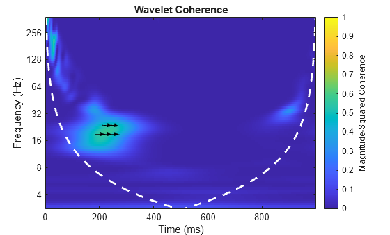
Use the pcolor command to plot the coherence and cone of influence.
figure
period = seconds(period);
coi = seconds(coi);
h = pcolor(t,log2(period),wcoh);
h.EdgeColor = "none";
ax = gca;
ytick=round(pow2(ax.YTick),3);
ax.YTickLabel=ytick;
ax.XLabel.String="Time";
ax.YLabel.String="Period";
ax.Title.String = "Wavelet Coherence";
hcol = colorbar;
hcol.Label.String = "Magnitude-Squared Coherence";
hold on
plot(ax,t,log2(coi),"w--",linewidth=2)
hold off

Use wcoherence(x,y,seconds(0.001)) without any output arguments. This plot includes the phase arrows and the cone of influence.
wcoherence(x,y,seconds(0.001))

Obtain the wavelet coherence for two signals. One signal consists of two sine waves of different frequencies in white noise. The sine waves have different time supports. The second signal is similar to the first, except it consists of two cosine waves.The sample rate is 1 kHz.
Set the random number generator to its default settings for reproducibility and create the two signals.
Fs = 1000;
rng default
t = 0:1/Fs:2;
x = cos(2*pi*10*t).*(t>=0.5 & t<1.1)+ ...
    cos(2*pi*50*t).*(t>= 0.2 & t< 1.4)+ ...
    0.25*randn(size(t));
y = sin(2*pi*10*t).*(t>=0.6 & t<1.2)+ ...
    sin(2*pi*50*t).*(t>= 0.4 & t<1.6)+ ...
    0.35*randn(size(t));
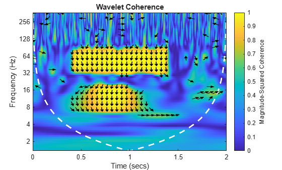
Visualize the wavelet coherence. The coherence plot is flipped with respect to the plot in the previous example, which specifies a sampling interval instead of a sampling frequency.
The phase is the phase delay of the second input, , with respect to the first input, . In this example, the is and the is . Since , the is a phase-delayed version of .
wcoherence(x,y,Fs)

If you swap the roles of and , then you see the phase at , because then and and or .
wcoherence(y,x,Fs)
Sample a sinusoid whose frequency is 8 Hz for 1 second. The sample rate is 1 kHz. Add noise to the signal.
Fs = 1000;
t = 0:1/Fs:1-1/Fs;
x = sin(8*2*pi*t) + 1/5*randn(1,length(t));
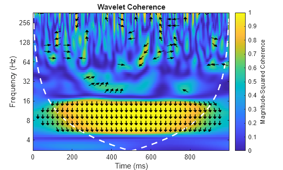
Sample a second sinusoid similar to the first sinusoid except introduce a phase shift of .
y = sin(8*2*pi*t+pi/2) + 1/5*randn(1,length(t));
Visualize the magnitude-squared wavelet coherence of the two signals. The direction of the arrows corresponds to the phase lag on the unit circle.
wcoherence(x,y,Fs)
Obtain the wavelet coherence for two signals sampled at 1000 Hz. One signal consists of two sine waves of different frequencies in white noise. The sine waves have different time supports. The second signal is similar to the first, except it consists of two cosine waves. Use the default number of scales to smooth. This value is equivalent to the number of voices per octave. Both values default to 12.
Set the random number generator to its default settings for reproducibility. Then, create the two signals and obtain the coherence.
rng default
Fs = 1000;
t = 0:1/Fs:2;
x = cos(2*pi*10*t).*(t>=0.5 & t<1.1)+ ...
    cos(2*pi*50*t).*(t>= 0.2 & t< 1.4)+ ...
    0.25*randn(size(t));
y = sin(2*pi*10*t).*(t>=0.6 & t<1.2)+ ...
    sin(2*pi*50*t).*(t>= 0.4 & t<1.6)+ ...
    0.35*randn(size(t));
wcoherence(x,y,Fs)

Set the number of scales to smooth to 18. The increased smoothing causes reduced low frequency resolution.
wcoherence(x,y,Fs,NumScalesToSmooth=18)

Compare the effects of using different phase display thresholds on the wavelet coherence.
Plot the wavelet coherence between the El Nino time series and the All India Average Rainfall Index. The data are sampled monthly. Specify the sampling interval as 1/12 of a year to display the periods in years. Use the default phase display threshold of 0.5, which shows phase arrows only where the coherence is greater than or equal to 0.5.
load ninoairdata
wcoherence(nino,air,years(1/12))
Set the phase display threshold to 0.7. Confirm the number of phase arrows decreases.
wcoherence(nino,air,years(1/12),PhaseDisplayThreshold=0.7);

Input Arguments
Name-Value Arguments
Output Arguments
More About
Tips
References
[1] Grinsted, A., J. C. Moore, and S. Jevrejeva. “Application of the Cross Wavelet Transform and Wavelet Coherence to Geophysical Time Series.” Nonlinear Processes in Geophysics 11, no. 5/6 (November 18, 2004): 561–66. https://doi.org/10.5194/npg-11-561-2004.
[2] Maraun, D., J. Kurths, and M. Holschneider. “Nonstationary Gaussian Processes in Wavelet Domain: Synthesis, Estimation, and Significance Testing.” Physical Review E 75, no. 1 (January 22, 2007): 016707. https://doi.org/10.1103/PhysRevE.75.016707.
[3] Torrence, Christopher, and Peter J. Webster. “Interdecadal Changes in the ENSO–Monsoon System.” Journal of Climate 12, no. 8 (August 1999): 2679–90. https://doi.org/10.1175/1520-0442(1999)012<2679:ICITEM>2.0.CO;2.