Resultados de

0 - 2 de 2

General

Athanasios Paraskevopoulos
Última actividad el 6 de Jun. de 2024

Numerical Simulation of the Discrete Klein-Gordon Equation: A Study on Damped, Driven Nonlinear Wave Systems with Spatially Extended Initial Conditions

The study of the dynamics of the discrete Klein - Gordon equation (DKG) with friction is given by the equation :

In the above equation, W describes the potential function:

to which every coupled unit

adheres. In Eq. (1), the variable $

$ is the unknown displacement of the oscillator occupying the n-th position of the lattice, and

is the discretization parameter. We denote by h the distance between the oscillators of the lattice. The chain (DKG) contains linear damping with a damping coefficient

, while

is the coefficient of the nonlinear cubic term.

For the DKG chain (1), we will consider the problem of initial-boundary values, with initial conditions

and Dirichlet boundary conditions at the boundary points

and

, that is,

Therefore, when necessary, we will use the short notation

for the one-dimensional discrete Laplacian

Now we want to investigate numerically the dynamics of the system (1)-(2)-(3). Our first aim is to conduct a numerical study of the property of Dynamic Stability of the system, which directly depends on the existence and linear stability of the branches of equilibrium points.

For the discussion of numerical results, it is also important to emphasize the role of the parameter

. By changing the time variable

, we rewrite Eq. (1) in the form

. We consider spatially extended initial conditions of the form:

where

is the distance of the grid and

is the amplitude of the initial condition

We also assume zero initial velocity:

the following graphs for

and

% Parameters
L = 200;  % Length of the system
K = 99;  % Number of spatial points
j = 2;  % Mode number
omega_d = 1;  % Characteristic frequency
beta = 1;  % Nonlinearity parameter
delta = 0.05;  % Damping coefficient
% Spatial grid
h = L / (K + 1);
n = linspace(-L/2, L/2, K+2);  % Spatial points
N = length(n);
omegaDScaled = h * omega_d;
deltaScaled = h * delta;
% Time parameters
dt = 1; % Time step
tmax = 3000; % Maximum time
tspan = 0:dt:tmax; % Time vector
% Values of amplitude 'a' to iterate over
a_values = [2, 1.95, 1.9, 1.85, 1.82];  % Modify this array as needed
% Differential equation solver function
function dYdt = odefun(~, Y, N, h, omegaDScaled, deltaScaled, beta)
    U = Y(1:N);
    Udot = Y(N+1:end);
    Uddot = zeros(size(U));
    % Laplacian (discrete second derivative)
    for k = 2:N-1
        Uddot(k) = (U(k+1) - 2 * U(k) + U(k-1)) ;
    end
    % System of equations
    dUdt = Udot;
    dUdotdt = Uddot - deltaScaled * Udot + omegaDScaled^2 * (U - beta * U.^3);
    % Pack derivatives
    dYdt = [dUdt; dUdotdt];
end
% Create a figure for subplots
figure;
% Initial plot
a_init = 2;  % Example initial amplitude for the initial condition plot
U0_init = a_init *  sin((j * pi * h * n) / L); % Initial displacement
U0_init(1) = 0; % Boundary condition at n = 0
U0_init(end) = 0; % Boundary condition at n = K+1
subplot(3, 2, 1);
plot(n, U0_init, 'r.-', 'LineWidth', 1.5, 'MarkerSize', 10); % Line and marker plot
xlabel('$x_n$', 'Interpreter', 'latex');
ylabel('$U_n$', 'Interpreter', 'latex');
title('$t=0$', 'Interpreter', 'latex');
set(gca, 'FontSize', 12, 'FontName', 'Times');
 xlim([-L/2 L/2]);
ylim([-3 3]);
grid on;
% Loop through each value of 'a' and generate the plot
for i = 1:length(a_values)
    a = a_values(i);
    % Initial conditions
    U0 = a * sin((j * pi * h * n) / L); % Initial displacement
    U0(1) = 0; % Boundary condition at n = 0
    U0(end) = 0; % Boundary condition at n = K+1
    Udot0 = zeros(size(U0)); % Initial velocity
    % Pack initial conditions
    Y0 = [U0, Udot0];
    % Solve ODE
    opts = odeset('RelTol', 1e-5, 'AbsTol', 1e-6);
    [t, Y] = ode45(@(t, Y) odefun(t, Y, N, h, omegaDScaled, deltaScaled, beta), tspan, Y0, opts);
    % Extract solutions
    U = Y(:, 1:N);
    Udot = Y(:, N+1:end);
    % Plot final displacement profile
    subplot(3, 2, i+1);
    plot(n, U(end,:), 'b.-', 'LineWidth', 1.5, 'MarkerSize', 10); % Line and marker plot
    xlabel('$x_n$', 'Interpreter', 'latex');
    ylabel('$U_n$', 'Interpreter', 'latex');
    title(['$t=3000$, $a=', num2str(a), '$'], 'Interpreter', 'latex');
    set(gca, 'FontSize', 12, 'FontName', 'Times');
      xlim([-L/2 L/2]);
ylim([-2 2]);
    grid on;
end
% Adjust layout
set(gcf, 'Position', [100, 100, 1200, 900]); % Adjust figure size as needed

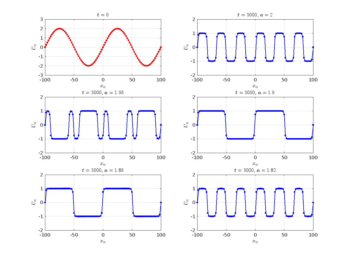
Dynamics for the initial condition ,

, for

, for different amplitude values. By reducing the amplitude values, we observe the convergence to equilibrium points of different branches from

and the appearance of values

for which the solution converges to a non-linear equilibrium point

Parameters:

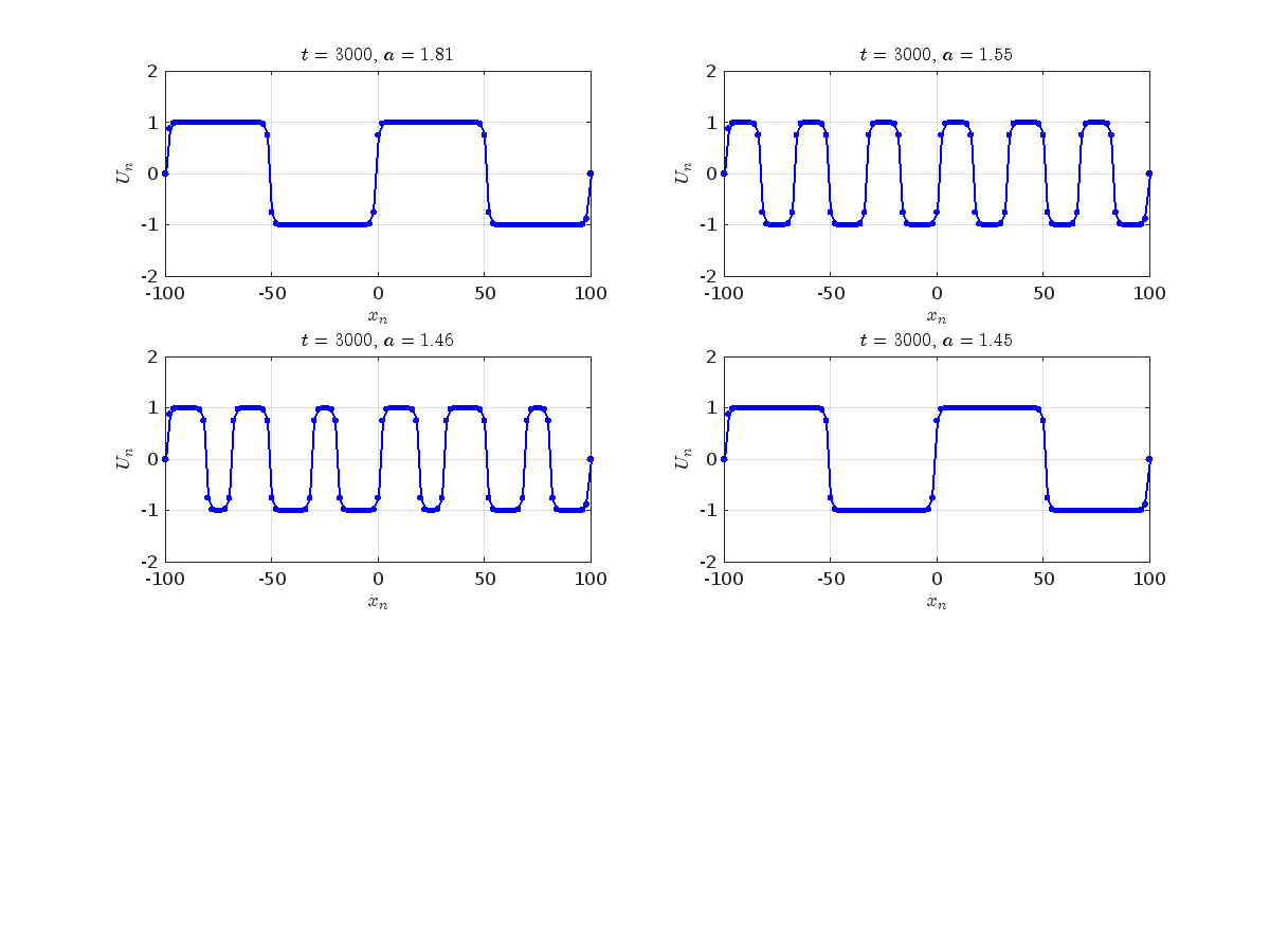
Detection of a stability threshold

: For

, the initial condition ,

, converges to a non-linear equilibrium point

Characteristics for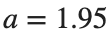

, with corresponding norm

where the dynamics appear in the first image of the third row, we observe convergence to a non-linear equilibrium point of branch

This has the same norm and the same energy as the previous case but the final state has a completely different profile. This result suggests secondary bifurcations have occurred in branch

By further reducing the amplitude, distinct values of

are discerned: 1.9, 1.85, 1.81 for which the initial condition

with norms

respectively, converges to a non-linear equilibrium point of branch

This equilibrium point has norm

and energy

. The behavior of this equilibrium is illustrated in the third row and in the first image of the third row of Figure 1, and also in the first image of the third row of Figure 2. For all the values between the aforementioned a, the initial condition

converges to geometrically different non-linear states of branch

as shown in the second image of the first row and the first image of the second row of Figure 2, for amplitudes

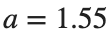and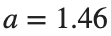

respectively.

Refference:

Dynamics of nonlinear lattices: asymptotic behavior and study of the existence and stability of tracked oscillations-Vetas Konstantinos (2018)

Ver publicación completa

General

Athanasios Paraskevopoulos
Última actividad el 5 de Mayo de 2024

Dynamic Simulation of DNA Base Pair Displacements with Non-linearity and Damping Effects

The study of the dynamics of the discrete Klein - Gordon equation (DKG) with friction is given by the equation :

above equation, W describes the potential function :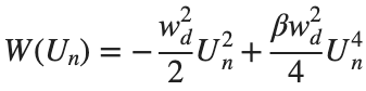

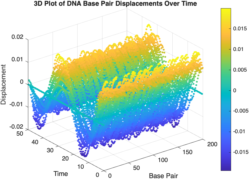
The objective of this simulation is to model the dynamics of a segment of DNA under thermal fluctuations with fixed boundaries using a modified discrete Klein-Gordon equation. The model incorporates elasticity, nonlinearity, and damping to provide insights into the mechanical behavior of DNA under various conditions.

% Parameters
numBases = 200; % Number of base pairs, representing a segment of DNA
kappa = 0.1; % Elasticity constant
omegaD = 0.2; % Frequency term
beta = 0.05; % Nonlinearity coefficient
delta = 0.01; % Damping coefficient

Position: Random initial perturbations between 0.01 and 0.02 to simulate the thermal fluctuations at the start.
Velocity: All bases start from rest, assuming no initial movement except for the thermal perturbations.

% Random initial perturbations to simulate thermal fluctuations
initialPositions = 0.01 + (0.02-0.01).*rand(numBases,1);
initialVelocities = zeros(numBases,1); % Assuming initial rest state

The simulation uses fixed ends to model the DNA segment being anchored at both ends, which is typical in experimental setups for studying DNA mechanics. The equations of motion for each base are derived from a modified discrete Klein-Gordon equation with the inclusion of damping:

% Define the differential equations
dt = 0.05; % Time step
tmax = 50; % Maximum time
tspan = 0:dt:tmax; % Time vector
x = zeros(numBases, length(tspan)); % Displacement matrix
x(:,1) = initialPositions; % Initial positions
% Velocity-Verlet algorithm for numerical integration
for i = 2:length(tspan)
    % Compute acceleration for internal bases
    acceleration = zeros(numBases,1);
    for n = 2:numBases-1
        acceleration(n) = kappa * (x(n+1, i-1) - 2 * x(n, i-1) + x(n-1, i-1)) ...
            - delta * initialVelocities(n) - omegaD^2 * (x(n, i-1) - beta * x(n, i-1)^3);
    end
    % positions for internal bases
    x(2:numBases-1, i) = x(2:numBases-1, i-1) + dt * initialVelocities(2:numBases-1) ...
        + 0.5 * dt^2 * acceleration(2:numBases-1);
    % velocities using new accelerations
    newAcceleration = zeros(numBases,1);
    for n = 2:numBases-1
        newAcceleration(n) = kappa * (x(n+1, i) - 2 * x(n, i) + x(n-1, i)) ...
            - delta * initialVelocities(n) - omegaD^2 * (x(n, i) - beta * x(n, i)^3);
    end
    initialVelocities(2:numBases-1) = initialVelocities(2:numBases-1) + 0.5 * dt * (acceleration(2:numBases-1) + newAcceleration(2:numBases-1));
end
% Visualization of displacement over time for each base pair
figure;
hold on;
for n = 2:numBases-1
    plot(tspan, x(n, :));
end
xlabel('Time');
ylabel('Displacement');
legend(arrayfun(@(n) ['Base ' num2str(n)], 2:numBases-1, 'UniformOutput', false));
title('Displacement of DNA Bases Over Time');
hold off;

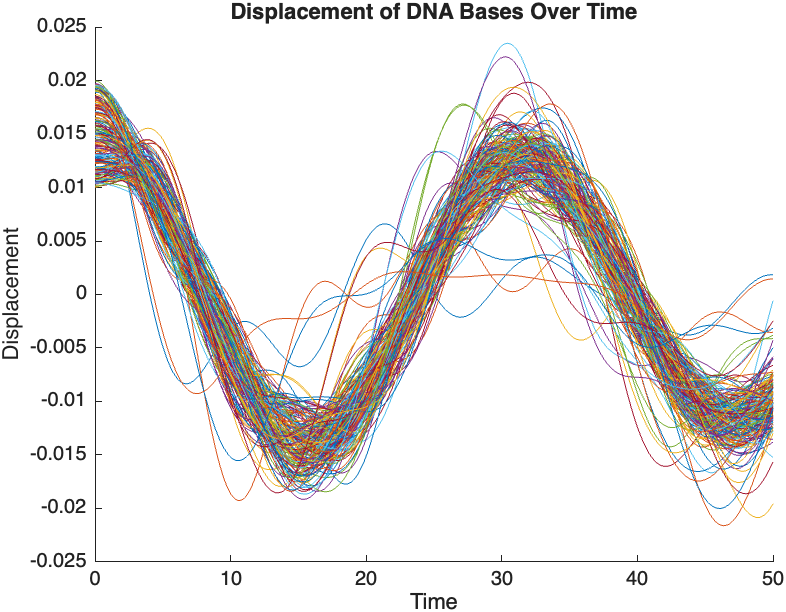
The results are visualized using a plot that shows the displacements of each base over time . Key observations from the simulation include :

Wave Propagation: The initial perturbations lead to wave-like dynamics along the segment, with visible propagation and reflection at the boundaries.
Damping Effects: The inclusion of damping leads to a gradual reduction in the amplitude of the oscillations, indicating energy dissipation over time.
Nonlinear Behavior: The nonlinear term influences the response, potentially stabilizing the system against large displacements or leading to complex dynamic patterns.

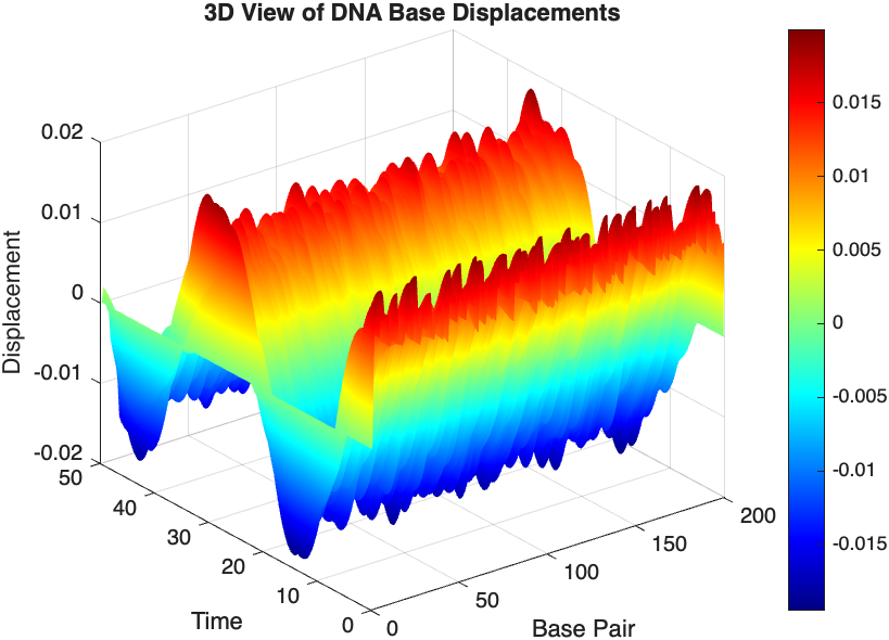
% 3D plot for displacement
figure;
[X, T] = meshgrid(1:numBases, tspan);
surf(X', T', x);
xlabel('Base Pair');
ylabel('Time');
zlabel('Displacement');
title('3D View of DNA Base Displacements');
colormap('jet');
shading interp;
colorbar; % Adds a color bar to indicate displacement magnitude

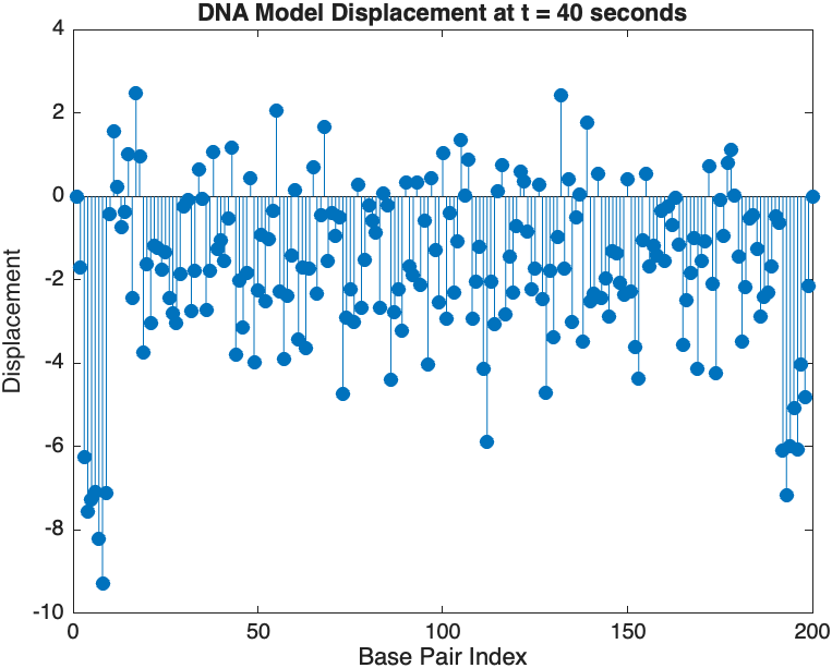
% Snapshot visualization at a specific time
snapshotTime = 40; % Desired time for the snapshot
[~, snapshotIndex] = min(abs(tspan - snapshotTime)); % Find closest index
snapshotSolution = x(:, snapshotIndex); % Extract displacement at the snapshot time
% Plotting the snapshot
figure;
stem(1:numBases, snapshotSolution, 'filled'); % Discrete plot using stem
title(sprintf('DNA Model Displacement at t = %d seconds', snapshotTime));
xlabel('Base Pair Index');
ylabel('Displacement');

% Time vector for detailed sampling
tDetailed = 0:0.5:50; % Detailed time steps
% Initialize an empty array to hold the data
data = [];
% Generate the data for 3D plotting
for i = 1:numBases
    % Interpolate to get detailed solution data for each base pair
    detailedSolution = interp1(tspan, x(i, :), tDetailed);
    % Concatenate the current base pair's data to the main data array
    data = [data; repmat(i, length(tDetailed), 1), tDetailed', detailedSolution'];
end
% 3D Plot
figure;
scatter3(data(:,1), data(:,2), data(:,3), 10, data(:,3), 'filled');
xlabel('Base Pair');
ylabel('Time');
zlabel('Displacement');
title('3D Plot of DNA Base Pair Displacements Over Time');
colorbar; % Adds a color bar to indicate displacement magnitude

Ver publicación completa

0 - 2 de 2