Resultados de
The study of the dynamics of the discrete Klein - Gordon equation (DKG) with friction is given by the equation :

above equation, W describes the potential function :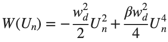
The objective of this simulation is to model the dynamics of a segment of DNA under thermal fluctuations with fixed boundaries using a modified discrete Klein-Gordon equation. The model incorporates elasticity, nonlinearity, and damping to provide insights into the mechanical behavior of DNA under various conditions.
% Parameters
numBases = 200; % Number of base pairs, representing a segment of DNA
kappa = 0.1; % Elasticity constant
omegaD = 0.2; % Frequency term
beta = 0.05; % Nonlinearity coefficient
delta = 0.01; % Damping coefficient
- Position: Random initial perturbations between 0.01 and 0.02 to simulate the thermal fluctuations at the start.
- Velocity: All bases start from rest, assuming no initial movement except for the thermal perturbations.
% Random initial perturbations to simulate thermal fluctuations
initialPositions = 0.01 + (0.02-0.01).*rand(numBases,1);
initialVelocities = zeros(numBases,1); % Assuming initial rest state
The simulation uses fixed ends to model the DNA segment being anchored at both ends, which is typical in experimental setups for studying DNA mechanics. The equations of motion for each base are derived from a modified discrete Klein-Gordon equation with the inclusion of damping:
% Define the differential equations
dt = 0.05; % Time step
tmax = 50; % Maximum time
tspan = 0:dt:tmax; % Time vector
x = zeros(numBases, length(tspan)); % Displacement matrix
x(:,1) = initialPositions; % Initial positions
% Velocity-Verlet algorithm for numerical integration
for i = 2:length(tspan)
% Compute acceleration for internal bases
acceleration = zeros(numBases,1);
for n = 2:numBases-1
acceleration(n) = kappa * (x(n+1, i-1) - 2 * x(n, i-1) + x(n-1, i-1)) ...
- delta * initialVelocities(n) - omegaD^2 * (x(n, i-1) - beta * x(n, i-1)^3);
end
% positions for internal bases
x(2:numBases-1, i) = x(2:numBases-1, i-1) + dt * initialVelocities(2:numBases-1) ...
+ 0.5 * dt^2 * acceleration(2:numBases-1);
% velocities using new accelerations
newAcceleration = zeros(numBases,1);
for n = 2:numBases-1
newAcceleration(n) = kappa * (x(n+1, i) - 2 * x(n, i) + x(n-1, i)) ...
- delta * initialVelocities(n) - omegaD^2 * (x(n, i) - beta * x(n, i)^3);
end
initialVelocities(2:numBases-1) = initialVelocities(2:numBases-1) + 0.5 * dt * (acceleration(2:numBases-1) + newAcceleration(2:numBases-1));
end
% Visualization of displacement over time for each base pair
figure;
hold on;
for n = 2:numBases-1
plot(tspan, x(n, :));
end
xlabel('Time');
ylabel('Displacement');
legend(arrayfun(@(n) ['Base ' num2str(n)], 2:numBases-1, 'UniformOutput', false));
title('Displacement of DNA Bases Over Time');
hold off;
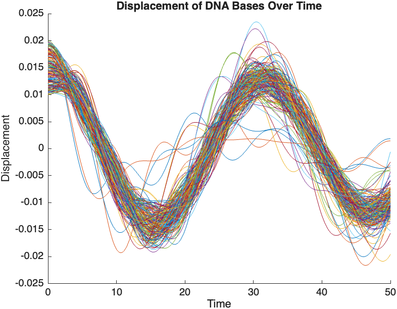
The results are visualized using a plot that shows the displacements of each base over time . Key observations from the simulation include :
- Wave Propagation: The initial perturbations lead to wave-like dynamics along the segment, with visible propagation and reflection at the boundaries.
- Damping Effects: The inclusion of damping leads to a gradual reduction in the amplitude of the oscillations, indicating energy dissipation over time.
- Nonlinear Behavior: The nonlinear term influences the response, potentially stabilizing the system against large displacements or leading to complex dynamic patterns.
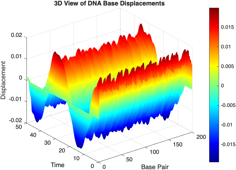
% 3D plot for displacement
figure;
[X, T] = meshgrid(1:numBases, tspan);
surf(X', T', x);
xlabel('Base Pair');
ylabel('Time');
zlabel('Displacement');
title('3D View of DNA Base Displacements');
colormap('jet');
shading interp;
colorbar; % Adds a color bar to indicate displacement magnitude
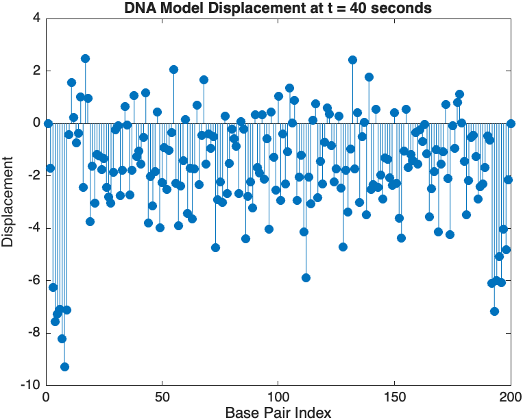
% Snapshot visualization at a specific time
snapshotTime = 40; % Desired time for the snapshot
[~, snapshotIndex] = min(abs(tspan - snapshotTime)); % Find closest index
snapshotSolution = x(:, snapshotIndex); % Extract displacement at the snapshot time
% Plotting the snapshot
figure;
stem(1:numBases, snapshotSolution, 'filled'); % Discrete plot using stem
title(sprintf('DNA Model Displacement at t = %d seconds', snapshotTime));
xlabel('Base Pair Index');
ylabel('Displacement');
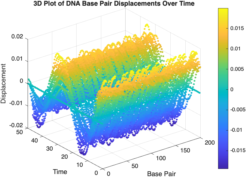
% Time vector for detailed sampling
tDetailed = 0:0.5:50; % Detailed time steps
% Initialize an empty array to hold the data
data = [];
% Generate the data for 3D plotting
for i = 1:numBases
% Interpolate to get detailed solution data for each base pair
detailedSolution = interp1(tspan, x(i, :), tDetailed);
% Concatenate the current base pair's data to the main data array
data = [data; repmat(i, length(tDetailed), 1), tDetailed', detailedSolution'];
end
% 3D Plot
figure;
scatter3(data(:,1), data(:,2), data(:,3), 10, data(:,3), 'filled');
xlabel('Base Pair');
ylabel('Time');
zlabel('Displacement');
title('3D Plot of DNA Base Pair Displacements Over Time');
colorbar; % Adds a color bar to indicate displacement magnitude
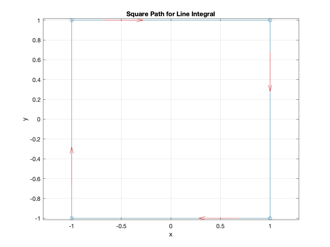
The line integral 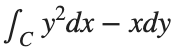 , where C is the boundary of the square
  oriented counterclockwise, can be evaluated in two ways:
, where C is the boundary of the square Using the definition of the line integral:
% Initialize the integral sum
integral_sum = 0;
% Segment C1: x = -1, y goes from -1 to 1
y = linspace(-1, 1);
x = -1 * ones(size(y));
dy = diff(y);
integral_sum = integral_sum + sum(-x(1:end-1) .* dy);
% Segment C2: y = 1, x goes from -1 to 1
x = linspace(-1, 1);
y = ones(size(x));
dx = diff(x);
integral_sum = integral_sum + sum(y(1:end-1).^2 .* dx);
% Segment C3: x = 1, y goes from 1 to -1
y = linspace(1, -1);
x = ones(size(y));
dy = diff(y);
integral_sum = integral_sum + sum(-x(1:end-1) .* dy);
% Segment C4: y = -1, x goes from 1 to -1
x = linspace(1, -1);
y = -1 * ones(size(x));
dx = diff(x);
integral_sum = integral_sum + sum(y(1:end-1).^2 .* dx);
disp(['Direct Method Integral: ', num2str(integral_sum)]);
Plotting the square path
% Define the square's vertices
vertices = [-1 -1; -1 1; 1 1; 1 -1; -1 -1];
% Plot the square
figure;
plot(vertices(:,1), vertices(:,2), '-o');
title('Square Path for Line Integral');
xlabel('x');
ylabel('y');
grid on;
axis equal;
% Add arrows to indicate the path direction (counterclockwise)
hold on;
for i = 1:size(vertices,1)-1
% Calculate direction
dx = vertices(i+1,1) - vertices(i,1);
dy = vertices(i+1,2) - vertices(i,2);
% Reduce the length of the arrow for better visibility
scale = 0.2;
dx = scale * dx;
dy = scale * dy;
% Calculate the start point of the arrow
startx = vertices(i,1) + (1 - scale) * dx;
starty = vertices(i,2) + (1 - scale) * dy;
% Plot the arrow
quiver(startx, starty, dx, dy, 'MaxHeadSize', 0.5, 'Color', 'r', 'AutoScale', 'off');
end
hold off;
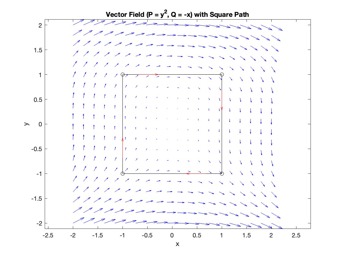
Apply Green's Theorem for the line integral
% Define the partial derivatives of P and Q
f = @(x, y) -1 - 2*y; % derivative of -x with respect to x is -1, and derivative of y^2 with respect to y is 2y
% Compute the double integral over the square [-1,1]x[-1,1]
integral_value = integral2(f, -1, 1, 1, -1);
disp(['Green''s Theorem Integral: ', num2str(integral_value)]);
Plotting the vector field related to Green’s theorem
% Define the grid for the vector field
[x, y] = meshgrid(linspace(-2, 2, 20), linspace(-2 ,2, 20));
% Define the vector field components
P = y.^2; % y^2 component
Q = -x; % -x component
% Plot the vector field
figure;
quiver(x, y, P, Q, 'b');
hold on; % Hold on to plot the square on the same figure
% Define the square's vertices
vertices = [-1 -1; -1 1; 1 1; 1 -1; -1 -1];
% Plot the square path
plot(vertices(:,1), vertices(:,2), '-o', 'Color', 'k'); % 'k' for black color
title('Vector Field (P = y^2, Q = -x) with Square Path');
xlabel('x');
ylabel('y');
axis equal;
% Add arrows to indicate the path direction (counterclockwise)
for i = 1:size(vertices,1)-1
% Calculate direction
dx = vertices(i+1,1) - vertices(i,1);
dy = vertices(i+1,2) - vertices(i,2);
% Reduce the length of the arrow for better visibility
scale = 0.2;
dx = scale * dx;
dy = scale * dy;
% Calculate the start point of the arrow
startx = vertices(i,1) + (1 - scale) * dx;
starty = vertices(i,2) + (1 - scale) * dy;
% Plot the arrow
quiver(startx, starty, dx, dy, 'MaxHeadSize', 0.5, 'Color', 'r', 'AutoScale', 'off');
end
hold off;
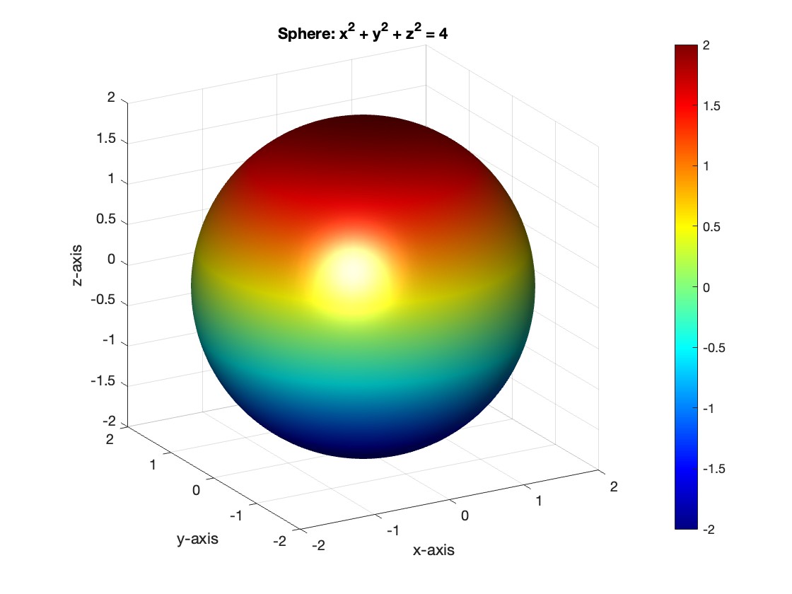
To solve a surface integral for example the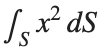 over the sphere
 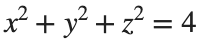 easily in MATLAB, you can leverage the symbolic toolbox for a direct and clear solution. Here is a tip to simplify the process:
over the sphere - Use Symbolic Variables and Functions: Define your variables symbolically, including the parameters of your spherical coordinates θ and ϕ and the radius r . This allows MATLAB to handle the expressions symbolically, making it easier to manipulate and integrate them.
- Express in Spherical Coordinates Directly: Since you already know the sphere's equation and the relationship in spherical coordinates, define x, y, and z in terms of r , θ and ϕ directly.
- Perform Symbolic Integration: Use MATLAB's `int` function to integrate symbolically. Since the sphere and the function
 are symmetric, you can exploit these symmetries to simplify the calculation.
Here’s how you can apply this tip in MATLAB code:
% Include the symbolic math toolbox
syms theta phi
% Define the limits for theta and phi
theta_limits = [0, pi];
phi_limits = [0, 2*pi];
% Define the integrand function symbolically
integrand = 16 * sin(theta)^3 * cos(phi)^2;
% Perform the symbolic integral for the surface integral
surface_integral = int(int(integrand, theta, theta_limits(1), theta_limits(2)), phi, phi_limits(1), phi_limits(2));
% Display the result of the surface integral symbolically
disp(['The surface integral of x^2 over the sphere is ', char(surface_integral)]);
% Number of points for plotting
num_points = 100;
% Define theta and phi for the sphere's surface
[theta_mesh, phi_mesh] = meshgrid(linspace(double(theta_limits(1)), double(theta_limits(2)), num_points), ...
linspace(double(phi_limits(1)), double(phi_limits(2)), num_points));
% Spherical to Cartesian conversion for plotting
r = 2; % radius of the sphere
x = r * sin(theta_mesh) .* cos(phi_mesh);
y = r * sin(theta_mesh) .* sin(phi_mesh);
z = r * cos(theta_mesh);
% Plot the sphere
figure;
surf(x, y, z, 'FaceColor', 'interp', 'EdgeColor', 'none');
colormap('jet'); % Color scheme
shading interp; % Smooth shading
camlight headlight; % Add headlight-type lighting
lighting gouraud; % Use Gouraud shading for smooth color transitions
title('Sphere: x^2 + y^2 + z^2 = 4');
xlabel('x-axis');
ylabel('y-axis');
zlabel('z-axis');
colorbar; % Add color bar to indicate height values
axis square; % Maintain aspect ratio to be square
view([-30, 20]); % Set a nice viewing angle
The study of nonlinear dynamical systems in lattices is an area of research with continuously growing interest.The first systematic studies of these systems emerged in the late 1930 s,thanks to the work of Frenkel and Kontorova on crystal dislocations.These studies led to the formulation of the discrete Klein-Gordon equation (DKG).Specifically,in 1939,Frenkel and Kontorova proposed a model that describes the structure and dynamics of a crystal lattice in a dislocation core.The FK model has become one of the fundamental models in physics,as it has been proven to reliably describe significant phenomena observed in discrete media.The equation we will examine is a variation of the following form:

The process described involves approximating a nonlinear differential equation through the Taylor method and simplifying it into a linear model.Let's analyze step by step the process from the initial equation to its final form.For small angles, can be approximated through the Taylor series as:
We substitute  in the original equation with the Taylor approximation:
To map this equation to a linear model,we consider the angles  to correspond to displacements
  in a mass-spring system.Thus,the equation transforms into:
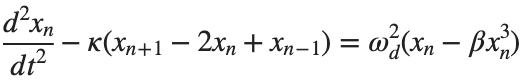
to correspond to displacements We recognize that the term  expresses the nonlinearity of the system,while β is a coefficient corresponding to this nonlinearity,simplifying the expression.The final form of the equation is:
The exact value of β depends on the mapping of coefficients in the Taylor approximation and its application to the specific physical problem.Our main goal is to derive results regarding stability and convergence in nonlinear lattices under nonlinear conditions.We will examine the basic characteristics of the discrete Klein-Gordon equation:
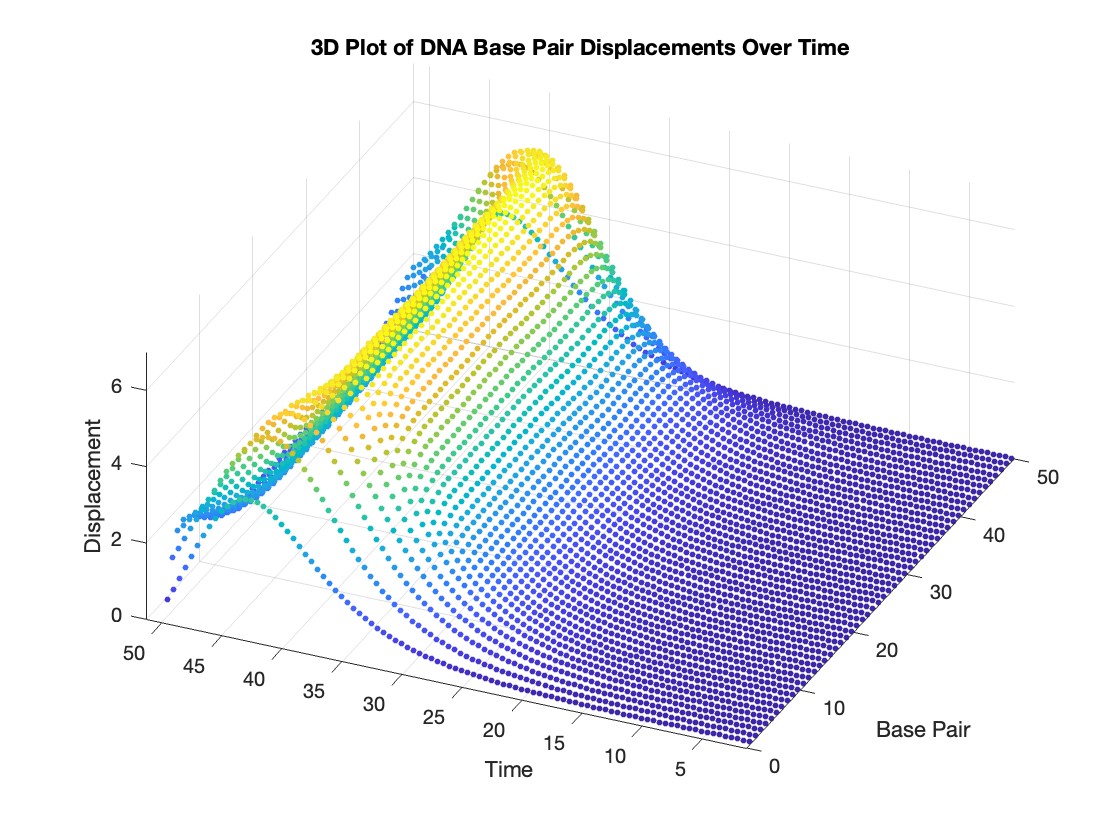
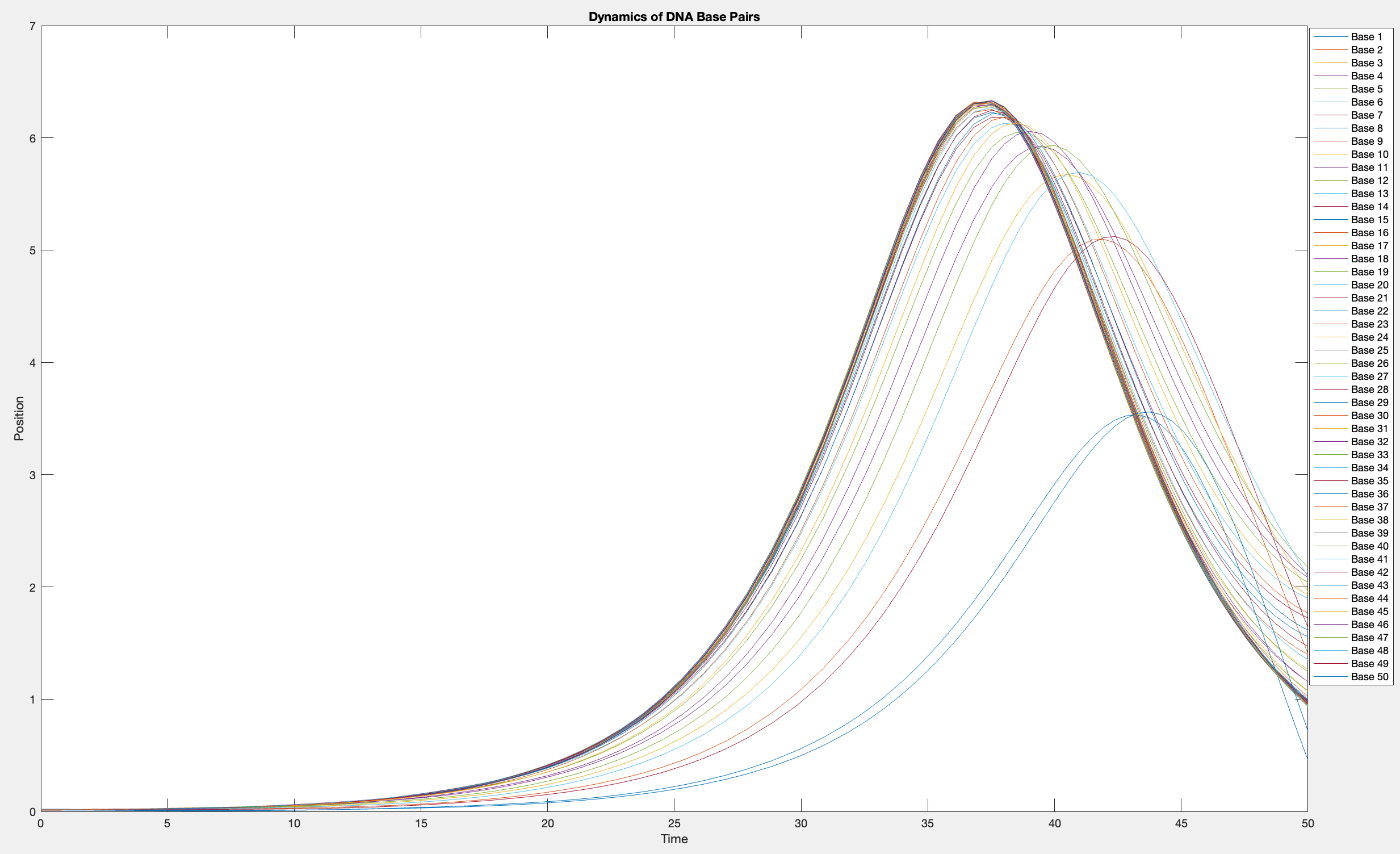
This model is often used to describe the opening of the DNA double helix during processes such as transcription.The model focuses on the transverse motion of the base pairs,which can be represented by a set of coupled nonlinear differential equations.
% Parameters
numBases = 50; % Number of base pairs
kappa = 0.1; % Elasticity constant
omegaD = 0.2; % Frequency term
beta = 0.05; % Nonlinearity coefficient
% Initial conditions
initialPositions = 0.01 + (0.02 - 0.01) * rand(numBases, 1);
initialVelocities = zeros(numBases, 1);
Time span
tSpan = [0 50];
>> % Differential equations
odeFunc = @(t, y) [y(numBases+1:end); ... % velocities
kappa * ([y(2); y(3:numBases); 0] - 2 * y(1:numBases) + [0; y(1:numBases-1)]) + ...
omegaD^2 * (y(1:numBases) - beta * y(1:numBases).^3)]; % accelerations
% Solve the system
[T, Y] = ode45(odeFunc, tSpan, [initialPositions; initialVelocities]);
% Visualization
plot(T, Y(:, 1:numBases))
legend(arrayfun(@(n) sprintf('Base %d', n), 1:numBases, 'UniformOutput', false))
xlabel('Time')
ylabel('Position')
title('Dynamics of DNA Base Pairs')
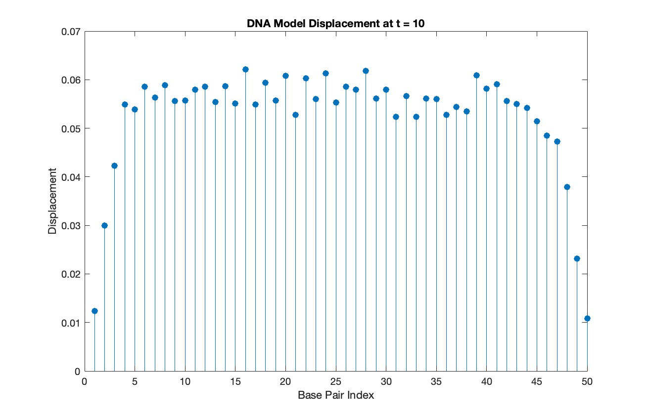
% Choose a specific time for the snapshot
snapshotTime = 10;
% Find the index in T that is closest to the snapshot time
[~, snapshotIndex] = min(abs(T - snapshotTime));
% Extract the solution at the snapshot time
snapshotSolution = Y(snapshotIndex, 1:numBases);
% Generate discrete plot for the DNA model at the snapshot time
figure;
stem(1:numBases, snapshotSolution, 'filled')
title(sprintf('DNA Model Displacement at t = %d', snapshotTime))
xlabel('Base Pair Index')
ylabel('Displacement')
% Time vector for detailed sampling
tDetailed = 0:0.5:50;
% Initialize an empty array to hold the data
data = [];
% Generate the data for 3D plotting
for i = 1:numBases
% Interpolate to get detailed solution data for each base pair
detailedSolution = interp1(T, Y(:, i), tDetailed);
% Concatenate the current base pair's data to the main data array
data = [data; repmat(i, length(tDetailed), 1), tDetailed', detailedSolution'];
end
% 3D Plot
figure;
scatter3(data(:,1), data(:,2), data(:,3), 10, data(:,3), 'filled')
xlabel('Base Pair')
ylabel('Time')
zlabel('Displacement')
title('3D Plot of DNA Base Pair Displacements Over Time')
colormap('rainbow')
colorbar