importNetworkFromPyTorch
Sintaxis
Descripción
Add-On Required: Esta funcionalidad requiere el
net = importNetworkFromPyTorch(modelfile)modelfile. La función devuelve la red net como un objeto dlnetwork sin inicializar.
importNetworkFromPyTorch requiere el paquete de soporte Deep Learning Toolbox™ Converter for PyTorch Models. Si no se ha instalado este paquete de soporte, importNetworkFromPyTorch proporciona un enlace de descarga.
Nota
La función importNetworkFromPyTorch puede generar una capa personalizada al importar una capa de PyTorch. Para obtener más información, consulte Algoritmos. Las funciones guardan las capas personalizadas generadas en el espacio de nombres +modelfile.
net = importNetworkFromPyTorch(modelfile,Name=Value)Namespace="CustomLayers" guarda las capas personalizadas generadas y las funciones asociadas en el espacio de nombres +CustomLayers de la carpeta actual. Si se ha especificado el argumento nombre-valor PyTorchInputSizes, la función podría devolver la red net como un objeto dlnetwork inicializado.
Para obtener más información sobre cómo rastrear un modelo de PyTorch, consulte https://pytorch.org/docs/stable/generated/torch.jit.trace.html.
Ejemplos
Importe un modelo de PyTorch preentrenado y rastreado como un objeto dlnetwork sin inicializar. Después, añada una capa de entrada en la red importada.
En este ejemplo se importa el modelo MNASNet (Copyright© Soumith Chintala 2016) de PyTorch. MNASNet es un modelo de clasificación de imágenes que se entrena con imágenes de la base de datos de ImageNet. Descargue el archivo mnasnet1_0, que tiene un tamaño aproximado de 17 MB, desde el sitio web de MathWorks.
modelfile = matlab.internal.examples.downloadSupportFile("nnet", ...
    "data/PyTorchModels/mnasnet1_0.pt");
Importe el modelo MNASNet usando la función importNetworkFromPyTorch. La función importa el modelo como un objeto dlnetwork sin inicializar sin capa de entrada. El software muestra una advertencia con información sobre el número de capas de entrada, el tipo de capa de entrada que se desea añadir y cómo añadir una capa de entrada.
net = importNetworkFromPyTorch(modelfile)
Warning: Network was imported as an uninitialized dlnetwork. Before using the network, add input layer(s):

% Create imageInputLayer for the network input at index 1:
inputLayer1 = imageInputLayer(<inputSize1>, Normalization="none");

% Add input layers to the network and initialize:
net = addInputLayer(net, inputLayer1, Initialize=true);
net =
  dlnetwork with properties:

         Layers: [3×1 nnet.cnn.layer.Layer]
    Connections: [2×2 table]
     Learnables: [210×3 table]
          State: [104×3 table]
     InputNames: {'TopLevelModule:layers'}
    OutputNames: {'TopLevelModule:classifier'}
    Initialized: 0

  View summary with summary.
Especifique el tamaño de entrada de la red importada y cree una capa de entrada de imágenes. Después, añada la capa de entrada de imágenes a la red importada e inicialice la red con la función addInputLayer.
InputSize = [224 224 3];
inputLayer = imageInputLayer(InputSize,Normalization="none");
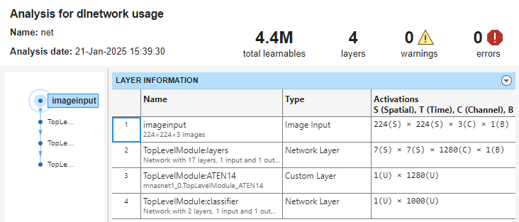
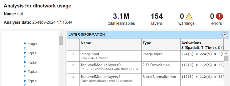
net = addInputLayer(net,inputLayer,Initialize=true);Analice la red importada y visualice la capa de entrada. La red se puede usar para hacer predicciones.
analyzeNetwork(net)
Importe un modelo de PyTorch preentrenado y rastreado como un objeto dlnetwork inicializado usando el argumento nombre-valor PyTorchInputSizes.
En este ejemplo se importa el modelo MNASNet (Copyright© Soumith Chintala 2016) de PyTorch. MNASNet es un modelo de clasificación de imágenes que se entrena con imágenes de la base de datos de ImageNet. Descargue el archivo mnasnet1_0.pt, que tiene un tamaño aproximado de 17 MB, desde el sitio web de MathWorks.
modelfile = matlab.internal.examples.downloadSupportFile("nnet", ...
    "data/PyTorchModels/mnasnet1_0.pt");
Importe el modelo MNASNet usando la función importNetworkFromPyTorch con el argumento nombre-valor PyTorchInputSizes. Sabemos que una imagen en color de 224x224 es un tamaño de entrada válido para este modelo de PyTorch. El software crea y añade automáticamente la capa de entrada para un lote de imágenes. Esto permite importar la red como una red inicializada usando una sola línea de código.
net = importNetworkFromPyTorch(modelfile,PyTorchInputSizes=[NaN,3,224,224])
net =
  dlnetwork with properties:

         Layers: [4×1 nnet.cnn.layer.Layer]
    Connections: [3×2 table]
     Learnables: [210×3 table]
          State: [104×3 table]
     InputNames: {'InputLayer1'}
    OutputNames: {'TopLevelModule:classifier'}
    Initialized: 1

  View summary with summary.
La red se puede usar para hacer predicciones.
Importe un modelo de PyTorch preentrenado y rastreado como un objeto dlnetwork sin inicializar. Después, inicialice la red importada.
En este ejemplo se importa el modelo MNASNet (Copyright© Soumith Chintal 2016) de PyTorch. MNASNet es un modelo de clasificación de imágenes que se entrena con imágenes de la base de datos de ImageNet. Descargue el archivo mnasnet1_0, que tiene un tamaño aproximado de 17 MB, desde el sitio web de MathWorks.
modelfile = matlab.internal.examples.downloadSupportFile("nnet", ...
    "data/PyTorchModels/mnasnet1_0.pt");
Importe el modelo MNASNet usando la función importNetworkFromPyTorch. La función importa el modelo como un objeto dlnetwork sin inicializar.
net = importNetworkFromPyTorch(modelfile)
Warning: Network was imported as an uninitialized dlnetwork. Before using the network, add input layer(s):

% Create imageInputLayer for the network input at index 1:
inputLayer1 = imageInputLayer(<inputSize1>, Normalization="none");

% Add input layers to the network and initialize:
net = addInputLayer(net, inputLayer1, Initialize=true);
net =
  dlnetwork with properties:

         Layers: [3×1 nnet.cnn.layer.Layer]
    Connections: [2×2 table]
     Learnables: [210×3 table]
          State: [104×3 table]
     InputNames: {'TopLevelModule:layers'}
    OutputNames: {'TopLevelModule:classifier'}
    Initialized: 0

  View summary with summary.
net es un objeto dlnetwork que consta de una sola capa networkLayer que contiene una red anidada. Especifique el tamaño de entrada de net y cree un objeto dlarray aleatorio que represente la entrada de la red. El formato de datos del objeto dlarray debe tener las dimensiones "SSCB" (espacial, espacial, canal, lote) para representar una entrada de imágenes 2D. Para obtener más información, consulte Data Formats for Prediction with dlnetwork.
InputSize = [224 224 3];
X = dlarray(rand(InputSize),"SSCB");
Inicialice los parámetros que se pueden aprender de la red importada usando la función initialize.
net = initialize(net,X);
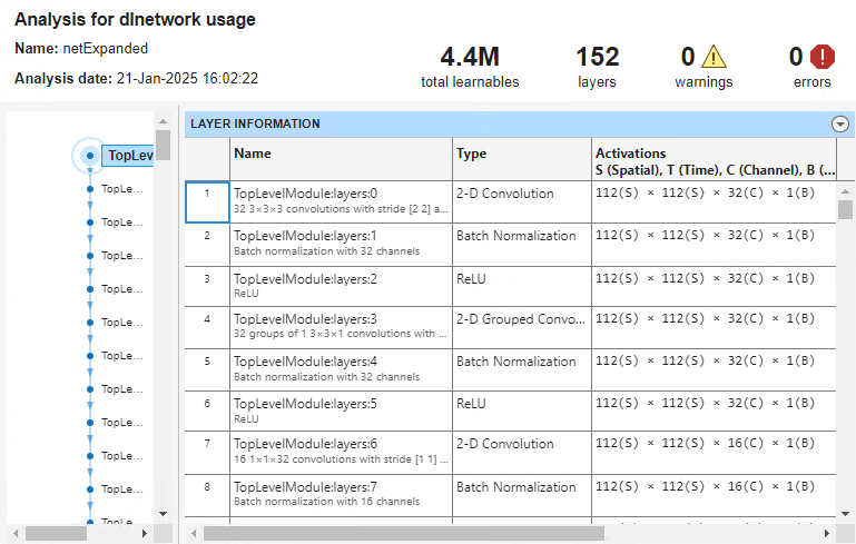
De este modo, la red importada está lista para hacer predicciones. Expanda networkLayer usando la función expandLayers y analice la red importada.
netExpanded = expandLayers(net)
netExpanded =
  dlnetwork with properties:

         Layers: [152×1 nnet.cnn.layer.Layer]
    Connections: [161×2 table]
     Learnables: [210×3 table]
          State: [104×3 table]
     InputNames: {'TopLevelModule:layers:0'}
    OutputNames: {'TopLevelModule:classifier:1:ATEN12'}
    Initialized: 1

  View summary with summary.
analyzeNetwork(netExpanded)
Importe un modelo de PyTorch preentrenado y rastreado como un objeto dlnetwork sin inicializar para clasificar una imagen.
En este ejemplo se importa el modelo MNASNet (Copyright© Soumith Chintala 2016) de PyTorch. MNASNet es un modelo de clasificación de imágenes que se entrena con imágenes de la base de datos de ImageNet. Descargue el archivo mnasnet1_0, que tiene un tamaño aproximado de 17 MB, desde el sitio web de MathWorks.
modelfile = matlab.internal.examples.downloadSupportFile("nnet", ...
    "data/PyTorchModels/mnasnet1_0.pt");
Importe el modelo MNASNet usando la función importNetworkFromPyTorch. La función importa el modelo como un objeto dlnetwork sin inicializar.
net = importNetworkFromPyTorch(modelfile)
Warning: Network was imported as an uninitialized dlnetwork. Before using the network, add input layer(s):

% Create imageInputLayer for the network input at index 1:
inputLayer1 = imageInputLayer(<inputSize1>, Normalization="none");

% Add input layers to the network and initialize:
net = addInputLayer(net, inputLayer1, Initialize=true);
net =
  dlnetwork with properties:

         Layers: [3×1 nnet.cnn.layer.Layer]
    Connections: [2×2 table]
     Learnables: [210×3 table]
          State: [104×3 table]
     InputNames: {'TopLevelModule:layers'}
    OutputNames: {'TopLevelModule:classifier'}
    Initialized: 0

  View summary with summary.
Especifique el tamaño de entrada de la red importada y cree una capa de entrada de imágenes. Después, añada la capa de entrada de imágenes a la red importada e inicialice la red con la función addInputLayer.
InputSize = [224 224 3];
inputLayer = imageInputLayer(InputSize,Normalization="none");
net = addInputLayer(net,inputLayer,Initialize=true);
Lea la imagen que desea clasificar.
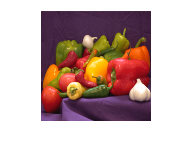
Im = imread("peppers.png");Cambie el tamaño de la imagen para que coincida con el tamaño de entrada de la red. Muestre la imagen.
InputSize = [224 224 3];
Im = imresize(Im,InputSize(1:2));
imshow(Im)
Las entradas de MNASNet requieren más procesamiento. Vuelva a escalar la imagen. Después, normalice la imagen restando la media de las imágenes de entrenamiento y dividiendo por la desviación estándar de las imágenes de entrenamiento. Para obtener más información, consulte Input Data Preprocessing.
Im = rescale(Im,0,1);

meanIm = [0.485 0.456 0.406];
stdIm = [0.229 0.224 0.225];
Im = (Im - reshape(meanIm,[1 1 3]))./reshape(stdIm,[1 1 3]);
Convierta la imagen en un objeto dlarray. Dé formato a la imagen con las dimensiones "SSCB" (espacial, espacial, canal, lote).
Im_dlarray = dlarray(single(Im),"SSCB");Obtenga los nombres de clase de squeezenet, que también se entrena con las imágenes de ImageNet.
[~,ClassNames] = imagePretrainedNetwork("squeezenet");Clasifique la imagen y encuentre la etiqueta predicha.
prob = predict(net,Im_dlarray);
[~,label_ind] = max(prob);
Muestre el resultado de la clasificación.
ClassNames(label_ind)
ans =
"bell pepper"
Importe un modelo de PyTorch preentrenado y rastreado como un objeto dlnetwork sin inicializar. Después, encuentre las capas personalizadas que genera el software.
En este ejemplo se usa la función de ayuda findCustomLayers.
En este ejemplo se importa el modelo MNASNet (Copyright© Soumith Chintala 2016) de PyTorch. MNASNet es un modelo de clasificación de imágenes que se entrena con imágenes de la base de datos de ImageNet. Descargue el archivo mnasnet1_0, que tiene un tamaño aproximado de 17 MB, desde el sitio web de MathWorks.
modelfile = matlab.internal.examples.downloadSupportFile("nnet", ...
    "data/PyTorchModels/mnasnet1_0.pt");
Importe el modelo MNASNet usando la función importNetworkFromPyTorch. La función importa el modelo como un objeto dlnetwork sin inicializar.
net = importNetworkFromPyTorch(modelfile)
Warning: Network was imported as an uninitialized dlnetwork. Before using the network, add input layer(s):

% Create imageInputLayer for the network input at index 1:
inputLayer1 = imageInputLayer(<inputSize1>, Normalization="none");

% Add input layers to the network and initialize:
net = addInputLayer(net, inputLayer1, Initialize=true);
net =
  dlnetwork with properties:

         Layers: [3×1 nnet.cnn.layer.Layer]
    Connections: [2×2 table]
     Learnables: [210×3 table]
          State: [104×3 table]
     InputNames: {'TopLevelModule:layers'}
    OutputNames: {'TopLevelModule:classifier'}
    Initialized: 0

  View summary with summary.
net es un objeto dlnetwork que consta de una sola capa networkLayer que contiene una red anidada. Expanda las capas de red anidada con la función expandLayers.
net = expandLayers(net);
La función importNetworkFromPyTorch genera capas personalizadas para las capas de PyTorch que la función no puede convertir en capas o funciones de MATLAB integradas. Para obtener más información, consulte Algoritmos. El software guarda las capas personalizadas generadas automáticamente en el espacio de nombres +mnasnet1_0 de la carpeta actual y las funciones asociadas en el espacio de nombres interno +ops. Para ver las capas personalizadas y las funciones asociadas, inspeccione el espacio de nombres.
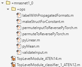
También puede encontrar los índices de las capas personalizadas generadas con la función de ayuda findCustomLayers. Muestre las capas personalizadas.
ind = findCustomLayers(net.Layers,'+mnasnet1_0')ind = 1×2
150 152
net.Layers(ind)
ans =
  2×1 Layer array with layers:

     1   'TopLevelModule:ATEN14'                Custom Layer   mnasnet1_0.TopLevelModule_ATEN14
     2   'TopLevelModule:classifier:1:ATEN12'   Custom Layer   mnasnet1_0.TopLevelModule_classifier_1_ATEN12
Función de ayuda
La función de ayuda findCustomLayers devuelve un vector lógico correspondiente a los indices de las capas personalizadas que importNetworkFromPyTorch genera automáticamente.
function indices = findCustomLayers(layers,Namespace)

s = what(['.' filesep Namespace]);

indices = zeros(1,length(s.m));
for i = 1:length(layers)
    for j = 1:length(s.m)
        if strcmpi(class(layers(i)),[Namespace(2:end) '.' s.m{j}(1:end-2)])
            indices(j) = i;
        end
    end
end

end
En este ejemplo se muestra cómo importar una red de PyTorch y entrenar la red para clasificar imágenes nuevas. Utilice la función importNetworkFromPytorch para importar la red como un objeto dlnetwork sin inicializar. Entrene la red con un bucle de entrenamiento personalizado.
En este ejemplo se usan las funciones de ayuda modelLoss, modelPredictions y preprocessMiniBatchPredictors.
En este ejemplo también se utiliza el archivo de soporte new_fcLayer. Para acceder al archivo de soporte, abra el ejemplo en Live Editor.
Cargar datos
Descomprima el conjunto de datos de MerchData, que contiene 75 imágenes. Cargue las nuevas imágenes como un almacén de datos de imágenes. La función imageDatastore etiqueta automáticamente las imágenes en función de los nombres de carpeta y almacena los datos como un objeto ImageDatastore. Divida los datos en conjuntos de datos de entrenamiento y de validación. Utilice el 70% de las imágenes para el entrenamiento y el 30% para la validación.
unzip("MerchData.zip");imds = imageDatastore("MerchData", ... IncludeSubfolders=true, ... LabelSource="foldernames"); [imdsTrain,imdsValidation] = splitEachLabel(imds,0.7);
La red usada en este ejemplo requiere imágenes de entrada de un tamaño de 224 por 224 por 3. Para cambiar automáticamente el tamaño de las imágenes de entrenamiento, utilice un almacén de datos de imágenes aumentado. Traslade aleatoriamente las imágenes hasta 30 píxeles en los ejes horizontal y vertical. El aumento de datos ayuda a evitar que la red se sobreajuste y memorice los detalles exactos de las imágenes de entrenamiento.
inputSize = [224 224 3];

pixelRange = [-30 30];
scaleRange = [0.9 1.1];
imageAugmenter = imageDataAugmenter(...
    RandXReflection=true, ...
    RandXTranslation=pixelRange, ...
    RandYTranslation=pixelRange, ...
    RandXScale=scaleRange, ...
    RandYScale=scaleRange);
augimdsTrain = augmentedImageDatastore(inputSize(1:2),imdsTrain, ...
    DataAugmentation=imageAugmenter);
Para cambiar el tamaño de las imágenes de validación de forma automática sin realizar más aumentos de datos, utilice un almacén de datos de imágenes aumentadas sin especificar ninguna operación adicional de preprocesamiento.
augimdsValidation = augmentedImageDatastore(inputSize(1:2),imdsValidation);
Determine el número de clases de los datos de entrenamiento.
classes = categories(imdsTrain.Labels);
numClasses = numel(classes);
Importar una red
Descargue el modelo MNASNet (Copyright© Soumith Chintala 2016) de PyTorch. MNASNet es un modelo de clasificación de imágenes que se entrena con imágenes de la base de datos de ImageNet. Descargue el archivo mnasnet1_0, que tiene un tamaño aproximado de 17 MB, desde el sitio web de MathWorks.
modelfile = matlab.internal.examples.downloadSupportFile("nnet", ...
    "data/PyTorchModels/mnasnet1_0.pt");
Importe el modelo MNASNet como un objeto dlnetwork sin inicializar usando la función importNetworkFromPyTorch.
net = importNetworkFromPyTorch(modelfile)
Warning: Network was imported as an uninitialized dlnetwork. Before using the network, add input layer(s):

% Create imageInputLayer for the network input at index 1:
inputLayer1 = imageInputLayer(<inputSize1>, Normalization="none");

% Add input layers to the network and initialize:
net = addInputLayer(net, inputLayer1, Initialize=true);
net =
  dlnetwork with properties:

         Layers: [3×1 nnet.cnn.layer.Layer]
    Connections: [2×2 table]
     Learnables: [210×3 table]
          State: [104×3 table]
     InputNames: {'TopLevelModule:layers'}
    OutputNames: {'TopLevelModule:classifier'}
    Initialized: 0

  View summary with summary.
net es un objeto dlnetwork que consta de una sola capa networkLayer que contiene una red anidada. Expanda networkLayer usando la función expandLayers. Muestre la capa final de la red importada usando la función analyzeNetwork.
net = expandLayers(net);
analyzeNetwork(net)
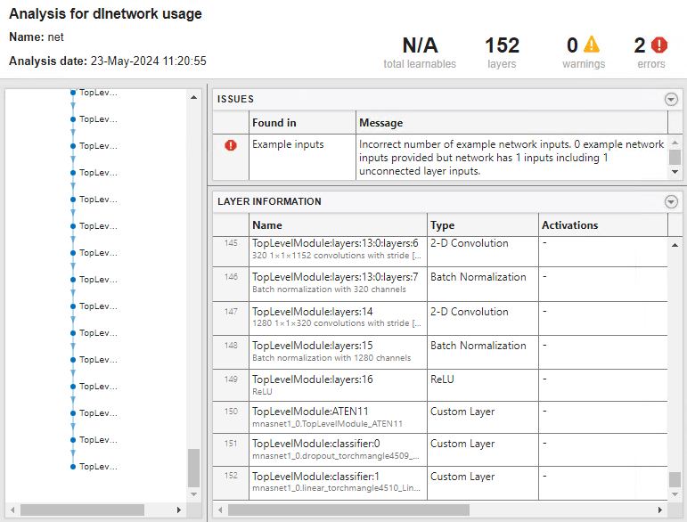
TopLevelModule:classifier:1:ATEN12 es una capa personalizada generada por la función importNetworkFromPyTorch y la última capa que se puede aprender de la red importada. Esta capa contiene información sobre cómo combinar las características que extrae la red en probabilidades de clase y un valor de pérdida.
Sustituir la capa final
Para volver a entrenar la red importada para clasificar imágenes nuevas, sustituya las capas finales por una nueva capa totalmente conectada. La nueva capa new_fclayer se adapta al nuevo conjunto de datos y también debe ser una capa personalizada porque tiene dos entradas.
Inicialice la capa new_fcLayer y sustituya la capa TopLevelModule:classifier:1:ATEN12 por new_fcLayer.
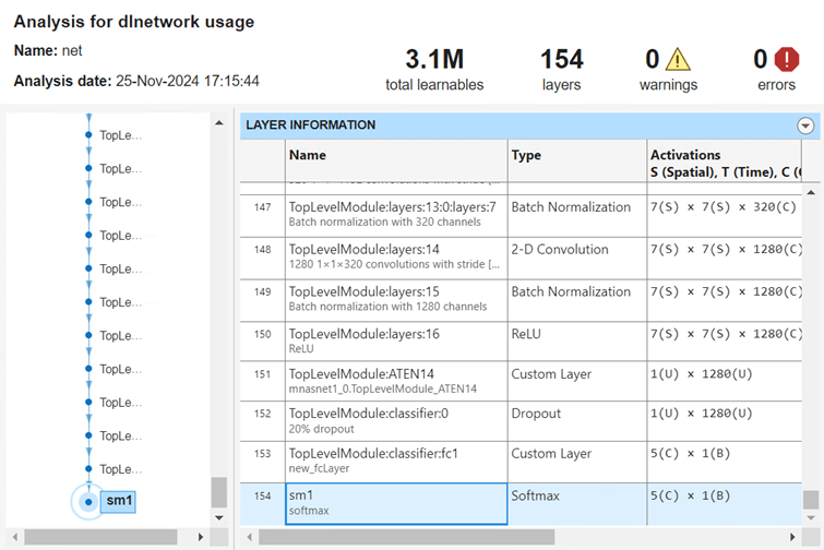
newLayer = new_fcLayer("TopLevelModule:classifier:fc1","Custom Layer", ...
    {'in'},{'out'},numClasses);
net = replaceLayer(net,"TopLevelModule:classifier:1:ATEN12",newLayer);
Añada una capa softmax a la red y conecte la capa softmax a la nueva capa totalmente conectada.
net = addLayers(net,softmaxLayer(Name="sm1"));
net = connectLayers(net,"TopLevelModule:classifier:fc1","sm1");
net.OutputNames = "sm1";
Añadir una capa de entrada
Añada una capa de entrada de imágenes a la red e inicialice la red.
inputLayer = imageInputLayer(inputSize,Normalization="none");
net = addInputLayer(net,inputLayer,Initialize=true);
Analice la red. Visualice la primera capa y las capas finales.
analyzeNetwork(net)
Definir la función de pérdida del modelo
El entrenamiento de una red neuronal profunda es una tarea de optimización. Tratando una red neuronal como si fuera una función , donde es la entrada de la red y es el conjunto de parámetros que se pueden aprender, puede optimizar para que minimice parte del valor de pérdida en función de los datos de entrenamiento. Por ejemplo, optimice los parámetros que se pueden aprender de modo que, para entradas con los objetivos correspondientes , minimicen el error entre las predicciones y .
Cree la función modelLoss, que aparece en la sección Función de pérdida del modelo del ejemplo, que toma como entrada el objeto dlnetwork y un minilote de datos de entrada con los objetivos correspondientes. La función devuelve la pérdida y los gradientes de la pérdida con respecto a los parámetros que se pueden aprender y el estado de la red.
Especificar las opciones de entrenamiento
Entrene con un tamaño de minilote de 20 durante 15 épocas.
numEpochs = 15;
miniBatchSize = 20;
Especifique las opciones para la optimización de SGDM. Especifique una tasa de aprendizaje inicial de 0,001 con un decaimiento de 0,005 y un momento de 0,9.
initialLearnRate = 0.001;
decay = 0.005;
momentum = 0.9;
Entrenar la red
Cree un objeto minibatchqueue que procese y gestione minilotes de imágenes durante el entrenamiento. Para cada minilote, siga estos pasos:
Utilice la función de preprocesamiento de minilotes personalizada
preprocessMiniBatch(definida al final de este ejemplo) para convertir las etiquetas en variables codificadas one-hot.Dé formato a los datos de imagen con las etiquetas de dimensión
"SSCB"(espacial, espacial, canal, lote). De forma predeterminada, el objetominibatchqueueconvierte los datos en objetosdlarraycon el tipo subyacentesingle. No dé formato a las etiquetas de clase.Entrene en una GPU, si se dispone de ella. De forma predeterminada, el objeto
minibatchqueueconvierte cada salida en un objetogpuArraysi hay una GPU disponible. Para utilizar una GPU se requiere una licencia de Parallel Computing Toolbox™ y un dispositivo GPU compatible. Para obtener información sobre los dispositivos compatibles, consulte GPU Computing Requirements (Parallel Computing Toolbox).
mbq = minibatchqueue(augimdsTrain,...
    MiniBatchSize=miniBatchSize,...
    MiniBatchFcn=@preprocessMiniBatch,...
    MiniBatchFormat=["SSCB" ""]);
Inicialice el parámetro de velocidad para el solver de gradiente descendente con momento (SGDM).
velocity = [];
Calcule el número total de iteraciones para monitorizar el progreso del entrenamiento.
numObservationsTrain = numel(imdsTrain.Files);
numIterationsPerEpoch = ceil(numObservationsTrain/miniBatchSize);
numIterations = numEpochs*numIterationsPerEpoch;
Inicialice el objeto trainingProgressMonitor. Dado que el cronómetro empieza cuando crea el objeto de monitorización, cree el objeto inmediatamente después del bucle de entrenamiento.
monitor = trainingProgressMonitor(Metrics="Loss",Info=["Epoch","LearnRate"],XLabel="Iteration");
Entrene la red con un bucle de entrenamiento personalizado. Para cada época, cambie el orden de los datos y pase en bucle por minilotes de datos. Para cada minilote, siga estos pasos:
Evalúe la pérdida, los gradientes y el estado del modelo utilizando las funciones
dlfevalymodelLoss, y actualice el estado de la red.Determine la tasa de aprendizaje para la programación de la tasa de aprendizaje de decaimiento basado en el tiempo.
Actualice los parámetros de red con la función
sgdmupdate.Actualice la pérdida, la tasa de aprendizaje y los valores de época en la monitorización del progreso del entrenamiento.
Detenga el proceso si la propiedad
Stopse ha establecido como verdadero. El valor de la propiedadStopdel objetoTrainingProgressMonitorcambia atruecuando hace clic en el botón Stop.
epoch = 0;
iteration = 0;

% Loop over epochs.
while epoch < numEpochs && ~monitor.Stop

    epoch = epoch + 1;

    % Shuffle data.
    shuffle(mbq);

    % Loop over mini-batches.
    while hasdata(mbq) && ~monitor.Stop

        iteration = iteration + 1;

        % Read mini-batch of data.
        [X,T] = next(mbq);

        % Evaluate the model gradients, state, and loss using dlfeval and the
        % modelLoss function and update the network state.
        [loss,gradients,state] = dlfeval(@modelLoss,net,X,T);
        net.State = state;

        % Determine learning rate for time-based decay learning rate schedule.
        learnRate = initialLearnRate/(1 + decay*iteration);

        % Update the network parameters using the SGDM optimizer.
        [net,velocity] = sgdmupdate(net,gradients,velocity,learnRate,momentum);

        % Update the training progress monitor.
        recordMetrics(monitor,iteration,Loss=loss);
        updateInfo(monitor,Epoch=epoch,LearnRate=learnRate);
        monitor.Progress = 100*iteration/numIterations;
    end
end
Clasificar imágenes de validación
Pruebe la precisión de clasificación del modelo comparando las predicciones en un conjunto de validación con las etiquetas verdaderas.
Después del entrenamiento, para hacer predicciones sobre nuevos datos no se requieren etiquetas. Cree un objeto minibatchqueue que contenga solo los predictores de los datos de prueba:
Para ignorar las etiquetas para las pruebas, establezca el número de salidas de la cola de minilotes en 1.
Especifique el mismo tamaño de minilote utilizado para el entrenamiento.
Preprocese los predictores mediante la función
preprocessMiniBatchPredictors, que se enumera al final del ejemplo.Para la salida única del almacén de datos, especifique el formato de los minilotes
"SSCB"(espacial, espacial, canal, lote).
numOutputs = 1;

mbqTest = minibatchqueue(augimdsValidation,numOutputs, ...
    MiniBatchSize=miniBatchSize, ...
    MiniBatchFcn=@preprocessMiniBatchPredictors, ...
    MiniBatchFormat="SSCB");
Pase en bucle por los minilotes y clasifique las imágenes con la función modelPredictions, que se enumera al final del ejemplo.
YTest = modelPredictions(net,mbqTest,classes);
Evalúe la precisión de clasificación.
TTest = imdsValidation.Labels;
accuracy = mean(TTest == YTest)
Visualice las predicciones en una gráfica de confusión. Los valores grandes de la diagonal indican predicciones precisas para la clase correspondiente. Los valores grandes fuera de la diagonal indican una fuerte confusión entre las clases correspondientes.
figure
confusionchart(TTest,YTest)
Funciones de ayuda
Función de pérdida del modelo
La función modelLoss toma un objeto net de dlnetwork como entrada y un minilote de datos de entrada X con objetivos correspondientes T. La función devuelve la pérdida, los gradientes de la pérdida con respecto a los parámetros que se pueden aprender en net y el estado de la red. Para calcular los gradientes automáticamente, utilice la función dlgradient.
function [loss,gradients,state] = modelLoss(net,X,T)

% Forward data through network.
[Y,state] = forward(net,X);

% Calculate cross-entropy loss.
loss = crossentropy(Y,T);

% Calculate gradients of loss with respect to learnable parameters.
gradients = dlgradient(loss,net.Learnables);

end
Función de predicciones del modelo
La función modelPredictions toma como entrada un objeto dlnetwork net, un minibatchqueue de datos de entrada mbq y las clases de red. La función calcula las predicciones del modelo iterando sobre todos los datos en el objeto minibatchqueue. La función utiliza la función onehotdecode para encontrar la clase predicha con la puntuación más alta.
function Y = modelPredictions(net,mbq,classes)

Y = [];

% Loop over mini-batches.
while hasdata(mbq)
    X = next(mbq);

    % Make prediction.
    scores = predict(net,X);

    % Decode labels and append to output.
    labels = onehotdecode(scores,classes,1)';
    Y = [Y; labels];
end

end
Función de preprocesamiento de minilotes
La función preprocessMiniBatch preprocesa un minilote de predictores y etiquetas siguiendo estos pasos:
Preprocesa las imágenes usando la función
preprocessMiniBatchPredictors.Extrae los datos de la etiqueta del arreglo de celdas entrante y concatena el resultado en un arreglo categórico a lo largo de la segunda dimensión.
Hace una codificación one-hot de las etiquetas categóricas en arreglos numéricos. La codificación en la primera dimensión produce un arreglo codificado que coincide con la forma de la salida de la red.
function [X,T] = preprocessMiniBatch(dataX,dataT)

% Preprocess predictors.
X = preprocessMiniBatchPredictors(dataX);

% Extract label data from cell and concatenate.
T = cat(2,dataT{1:end});

% One-hot encode labels.
T = onehotencode(T,1);

end
Función de preprocesamiento de predictores de minilotes
La función preprocessMiniBatchPredictors preprocesa un minilote de predictores extrayendo los datos de imagen del arreglo de celdas de entrada y concatenando el resultado en un arreglo numérico. Para entradas en escala de grises, la concatenación sobre la cuarta dimensión añade una tercera dimensión a cada imagen, para usarla como dimensión de canal única.
function X = preprocessMiniBatchPredictors(dataX)

% Concatenate.
X = cat(4,dataX{1:end});

end
Argumentos de entrada
Argumentos de par nombre-valor
Argumentos de salida
Limitaciones
La función
importNetworkFromPyTorchpuede importar la mayoría de (aunque no todas) las redes creadas en versiones de PyTorch distintas a la versión 2.0. La función es totalmente compatible con la versión 2.0 de PyTorch.La función
importNetworkFromPyTorchno admite modelos de detección de objetos de PyTorch que contienen operadores de Torchvision.
Más acerca de
Sugerencias
Para usar una red preentrenada para predicción o transferencia del aprendizaje en imágenes nuevas, debe preprocesar las imágenes del mismo modo que las imágenes que use para entrenar el modelo importado. Los pasos de preprocesamiento más habituales son modificar el tamaño de las imágenes, restar los valores promedio de la imagen y convertir las imágenes de formato BGR a RGB.
Para obtener más información sobre las imágenes de preprocesamiento para entrenamiento y predicción, consulte Preprocesar imágenes para deep learning.
No es posible acceder a los miembros del espacio de nombres
+si la carpeta principal del espacio de nombres no está en la ruta de MATLAB. Para obtener más información, consulte Namespaces and the MATLAB Path.NamespaceMATLAB usa la indexación de base uno, mientras que Python usa la indexación de base cero. Es decir, el primer elemento de un arreglo tiene un índice de 1 y 0 en MATLAB y Python, respectivamente. Para obtener más información sobre la indexación de MATLAB, consulte Indexación de arreglos. En MATLAB, para usar un arreglo de índices (
ind) creado en Python, convierta el arreglo enind+1.Si encuentra un conflicto de biblioteca de Python, utilice la función
pyenvpara especificar el argumento nombre-valorExecutionModecomo"OutOfProcess".Para ver más consejos, consulte Tips on Importing Models from TensorFlow, PyTorch, and ONNX.
Algoritmos
La función importNetworkFromPyTorch importa una capa de PyTorch en MATLAB siguiendo por orden estos pasos:
La función trata de importar la capa de PyTorch como una capa de MATLAB integrada. Para obtener más información, consulte Conversión de capas de PyTorch.
La función trata de importar la capa de PyTorch como una función de MATLAB integrada. Para obtener más información, consulte Conversión de capas de PyTorch.
La función trata de importar la capa de PyTorch como una capa personalizada. La función
importNetworkFromPyTorchguarda las capas personalizadas generadas y las funciones asociadas en el espacio de nombres+. Para ver un ejemplo, consulte Importar redes de PyTorch y encontrar capas personalizadas generadas.NamespaceLa función importa la capa de PyTorch como una capa personalizada con una función de marcador de posición. Debe completar la función de marcador de posición antes de poder usar la red; consulte Funciones de marcador de posición.
En los tres primeros casos, la red importada está lista para la predicción después de inicializarla.
Funcionalidad alternativa
App
También puede importar redes de plataformas externas utilizando la app Deep Network Designer. La app utiliza la función importNetworkFromPyTorch para importar la red y muestra un cuadro de diálogo de progreso. Durante el proceso de importación, la app añade una capa de entrada a la red, si es posible, y muestra un informe de importación que incluye detalles sobre los problemas que requieren atención. Después de importar una red, puede editarla, visualizarla y analizarla de manera interactiva. Cuando termine de editar la red, puede exportarla a Simulink® o generar código de MATLAB para construir redes.
Bloque
También puede trabajar con redes de PyTorch utilizando el bloque PyTorch Model Predict. Este bloque también permite cargar funciones de Python para preprocesar o posprocesar datos, así como configurar puertos de entrada y salida de manera interactiva.
Historial de versiones
Introducido en R2022bConsulte también
importNetworkFromONNX | importNetworkFromTensorFlow | exportONNXNetwork | exportNetworkToTensorFlow | dlnetwork | dlarray | addInputLayer