Check Model Assumptions for Chow Test
This example shows how to check the model assumptions for a Chow test. The model is of U.S. gross domestic product (GDP), with consumer price index (CPI) and paid compensation of employees (COE) as predictors. The forecast horizon is 2007 - 2009, just before and after the 2008 U.S. recession began.
Load and Inspect Data
Load the U.S. macroeconomic data set.
load Data_USEconModelThe time series in the data set contain quarterly, macroeconomic measurements from 1947 to 2009. For more details, a list of variables, and descriptions, enter Description at the command line.
Extract the predictors and the response from the table. Focus the sample on observations taken from 1960 - 2009.
idx = year(DataTimeTable.Time) >= 1960;
dates = DataTimeTable.Time(idx);
y = DataTimeTable.GDP(idx);
X = DataTimeTable{idx,["CPIAUCSL" "COE"]};
varNames = ["CPIAUCSL" "COE" "GDP"];
Identify forecast horizon indices.
fHIdx = year(dates) >= 2007;
Plot all series individually. Identify the periods of recession.
figure
tiledlayout(2,2)
nexttile
plot(dates,y)
title(varNames{end});
xlabel("Year");
axis tight;
recessionplot;
for j = 1:size(X,2)
    nexttile
    plot(dates,X(:,j))
    title(varNames{j});
    xlabel("Year");
    axis tight;
    recessionplot;
end
All variables appear to grow exponentially. Also, around the last recession, a decline appears. Suppose that a linear regression model of GDP onto CPI and COE is appropriate, and you want to test whether there is a structural change in the model in 2007.
Check Chow Test Assumptions
Chow tests rely on:
Independent, Gaussian-distributed innovations
Constancy of the innovations variance within subsamples
Constancy of the innovations across any structural breaks
If a model violates these assumptions, then the Chow test result might not be correct, or the Chow test might lack power. Investigate whether the assumptions hold. If any do not, preprocess the data further.
Fit the linear model to the entire series. Include an intercept.
Mdl = fitlm(X,y);
Mdl is a LinearModel model object.
Draw two histogram plots using the residuals: one with respect to fitted values in case order, and the other with respect to the previous residual.
figure
tiledlayout(2,1)
nexttile
plotResiduals(Mdl,"lagged");
nexttile
plotResiduals(Mdl,"caseorder");
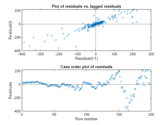
Because the scatter plot of residual vs. lagged residual forms a trend, autocorrelation exists in the residuals. Also, residuals on the extremes seem to flare out, which suggests the presence of heteroscedasticity.
Conduct Engle's ARCH test at 5% level of significance to assess whether the innovations have conditional heteroscedasticity with ARCH(1) effects. Supply the table of residuals and specify the raw residuals.
StatTbl = archtest(Mdl.Residuals,DataVariable="Raw")StatTbl=1×6 table
h pValue stat cValue Lags Alpha
_____ ______ ______ ______ ____ _____
Test 1 true 0 109.37 3.8415 1 0.05
h = 1 suggests to reject the null hypothesis that the entire residual series has no conditional heteroscedasticity.
Apply the log transformation to all series that appear to grow exponentially to reduce the effects of heteroscedasticity.
y = log(y);
X = log(X);
To account for autocorrelation, create predictor variables for all exponential series by lagging them by one period.
LagMat = lagmatrix([X y],1);
X = [X(2:end,:)  LagMat(2:end,:)]; % Concatenate data and remove first row
fHIdx = fHIdx(2:end);
y = y(2:end);
Based on the residual diagnostics, choose this linear model for GDP
should be a Gaussian series of innovations with mean zero and constant variance .
Diagnose the residuals again.
Mdl = fitlm(X,y);

figure
tiledlayout(2,1)
nexttile
plotResiduals(Mdl,"lagged");
nexttile
plotResiduals(Mdl,"caseorder");
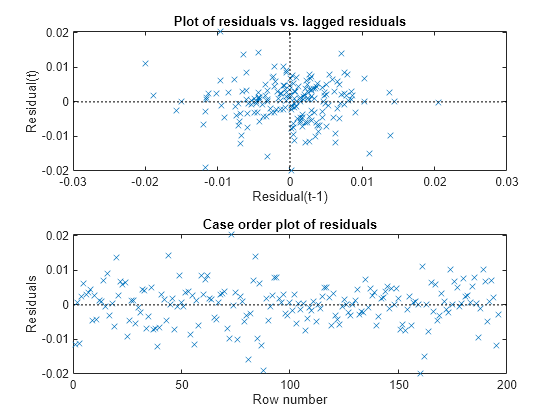
StatTbl = archtest(Mdl.Residuals,DataVariable="Raw")StatTbl=1×6 table
h pValue stat cValue Lags Alpha
_____ _______ ______ ______ ____ _____
Test 1 false 0.28133 1.1607 3.8415 1 0.05
SubMdl = {fitlm(X(~fHIdx,:),y(~fHIdx)) fitlm(X(fHIdx,:),y(fHIdx))};
subRes = {SubMdl{1}.Residuals.Raw SubMdl{2}.Residuals.Raw};
[hVT2,pValueVT2] = vartest2(subRes{1},subRes{2})
hVT2 = 0
pValueVT2 =
0.1645
The residual plots and tests suggest that the innovations are homoscedastic and uncorrelated.
Conduct a Kolmogorov-Smirnov test to assess whether the innovations are Gaussian.
[hKS,pValueKS] = kstest(Mdl.Residuals.Raw/std(Mdl.Residuals.Raw))
hKS = logical
   0
pValueKS =
0.2347
hKS = 0 suggests to not reject the null hypothesis that the innovations are Gaussian.
For the distributed lag model, the Chow test assumptions appear valid.
Conduct Chow Test
Treating 2007 and beyond as a post-recession regime, test whether the linear model is stable. Specify that the break point is the last quarter of 2006. Because the complementary subsample size is greater than the number of coefficients, conduct a break point test.
bp = find(~fHIdx,1,'last');
chowtest(X,y,bp,'Display','summary');
RESULTS SUMMARY

***************
Test 1

Sample size: 196
Breakpoint: 187

Test type: breakpoint
Coefficients tested: All

Statistic: 1.3741
Critical value: 2.1481

P value: 0.2272
Significance level: 0.0500

Decision: Fail to reject coefficient stability
The test fails to reject the stability of the linear model. Evidence is inefficient to infer a structural change between Q4-2006 and Q1-2007.
See Also
chowtest | archtest | vartest2 | fitlm | LinearModel