edr

Edit distance on real signals

Syntax

dist = edr(x,y,tol)

[dist,ix,iy] = edr(x,y,tol)

[___] = edr(x,y,maxsamp)

[___] = edr(___,metric)

edr(___)

Description

dist = edr(x,y,tol) returns the Edit Distance on Real Signals between sequences x and y. edr returns the minimum number of elements that must be removed from x, y, or both x and y, so that the sum of Euclidean distances between the remaining signal elements lies within the specified tolerance, tol.

[dist,ix,iy] = edr(x,y,tol) returns the warping path such that x(ix) and y(iy) have the smallest possible dist between them. When x and y are matrices, ix and iy are such that x(:,ix) and y(:,iy) are minimally separated.

[___] = edr(x,y,maxsamp) restricts the insertion operations so that the warping path remains within maxsamp samples of a straight-line fit between x and y. This syntax returns any of the output arguments of previous syntaxes.

[___] = edr(___,metric) specifies the distance metric to use in addition to any of the input arguments in previous syntaxes. metric can be one of 'euclidean', 'absolute', 'squared', or 'symmkl'.

edr(___) without output arguments plots the original and aligned signals.

• If the signals are real vectors, the function displays the two original signals on a subplot and the aligned signals in a subplot below the first one.

• If the signals are complex vectors, the function displays the original and aligned signals in three-dimensional plots.

• If the signals are real matrices, the function uses imagesc to display the original and aligned signals.

• If the signals are complex matrices, the function plots their real and imaginary parts in the top and bottom half of each image.

Examples

Edit Distance Between Chirp and Sinusoid with Outliers

Generate two real signals: a chirp and a sinusoid. Add a clearly outlying section to each signal.

x = cos(2*pi*(3*(1:1000)/1000).^2);
y = cos(2*pi*9*(1:399)/400);

x(400:410) = 7;
y(100:115) = 7;

Warp the signals so that the edit distance between them is smallest. Specify a tolerance of 0.1. Plot the aligned signals, both before and after the warping, and output the distance between them.

tol = 0.1;
edr(x,y,tol)

ans = 
617

Change the sinusoid frequency to twice its initial value. Repeat the computation.

y = cos(2*pi*18*(1:399)/400);
y(100:115) = 7;

edr(x,y,tol);

Add an imaginary part to each signal. Restore the initial sinusoid frequency. Align the signals by minimizing the sum of squared Euclidean distances.

x = exp(2i*pi*(3*(1:1000)/1000).^2);
y = exp(2i*pi*9*(1:399)/400);

x(400:405) = 5+3j;
x(405:410) = 7;

y(100:107) = 3j;
y(108:115) = 7-3j;

edr(x,y,tol,'squared');

Edit Distance and Warping Path

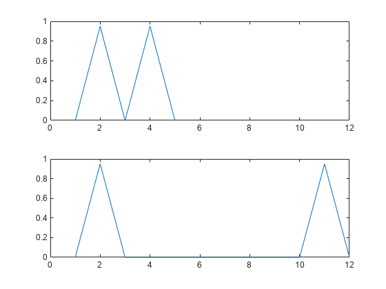
Generate two signals consisting of two distinct peaks separated by valleys of different lengths. Plot the signals.

x1 = [0 1 0 1 0]*.95;
x2 = [0 1 0 0 0 0 0 0 1 0]*.95;

subplot(2,1,1)
plot(x1)
xlim([0 12])
subplot(2,1,2)
plot(x2)
xlim([0 12])

Compute the edit distance between the signals. Set a small tolerance so that the only matches are between equal samples.

tol = 0.1;

figure
edr(x1,x2,tol);

The distance between the signals is 7. To align them, it is necessary to remove the seven central zeros of x2 or add seven zeros to x1.

Compute the D matrix, whose bottom-right element corresponds to the edit distance. For the definition of D, see Edit Distance on Real Signals.

cnd = (abs(x1'-x2))>tol;
D = zeros(length(x1)+1,length(x2)+1);
D(1,2:end) = 1:length(x2);
D(2:end,1) = 1:length(x1);

for h = 2:length(x1)+1
    for k = 2:length(x2)+1
        D(h,k) = min([D(h-1,k)+1 ...
            D(h,k-1)+1 ...
            D(h-1,k-1)+cnd(h-1,k-1)]);
    end
end

D

D = 6×11

     0     1     2     3     4     5     6     7     8     9    10
     1     0     1     2     3     4     5     6     7     8     9
     2     1     0     1     2     3     4     5     6     7     8
     3     2     1     0     1     2     3     4     5     6     7
     4     3     2     1     1     2     3     4     5     5     6
     5     4     3     2     1     1     2     3     4     5     5

Compute and display the warping path that aligns the signals.

[d,i1,i2] = edr(x1,x2,tol);

E = zeros(length(x1),length(x2));

for k = 1:length(i1)
    E(i1(k),i2(k)) = NaN;
end

E

E = 5×10

   NaN     0     0     0     0     0     0     0     0     0
     0   NaN     0     0     0     0     0     0     0     0
     0     0   NaN   NaN   NaN   NaN   NaN   NaN     0     0
     0     0     0     0     0     0     0     0   NaN     0
     0     0     0     0     0     0     0     0     0   NaN

Repeat the computation, but now constrain the warping path to deviate at most two elements from the diagonal. Plot the stretched signals and the warping path. In the second plot, set the matrix columns to run along the x-axis.

[dc,i1c,i2c] = edr(x1,x2,tol,2);

subplot(2,1,1)
plot([x1(i1c);x2(i2c)]','.-')
title(['Distance: ' num2str(dc)])
subplot(2,1,2)
plot(i2c,i1c,'o-',[i2(1) i2(end)],[i1(1) i1(end)])
axis ij
title('Warping Path')

The constraint results in a smaller edit distance but distorts the signals. If the constraint cannot be met, then edr returns NaN for the distance. See this by forcing the warping path to deviate at most one element from the diagonal.

[dc,i1c,i2c] = edr(x1,x2,tol,1);

subplot(2,1,1)
plot([x1(i1c);x2(i2c)]','.-')
title(['Distance: ' num2str(dc)])
subplot(2,1,2)
plot(i2c,i1c,'o-',[i2(1) i2(end)],[i1(1) i1(end)])
axis ij
title('Warping Path')

Align Blotched Handwriting Samples

The files MATLAB1.gif and MATLAB2.gif contain two handwritten samples of the word "MATLAB®." Load the files. Add outliers by blotching the data.

samp1 = 'MATLAB1.gif';
samp2 = 'MATLAB2.gif';

x = double(imread(samp1));
y = double(imread(samp2));

x(15:20,54:60) = 4000;
y(15:20,84:96) = 4000;

Align the handwriting samples along the x-axis using the edit distance. Specify a tolerance of 450.

edr(x,y,450);

Input Arguments

x — Input signal

vector | matrix

Input signal, specified as a real or complex vector or matrix.

Data Types: single | double
Complex Number Support: Yes

y — Input signal

vector | matrix

Input signal, specified as a real or complex vector or matrix.

Data Types: single | double
Complex Number Support: Yes

tol — Tolerance

positive scalar

Tolerance, specified as a positive scalar.

Data Types: single | double

maxsamp — Width of adjustment window

Inf (default) | positive integer

Width of adjustment window, specified as a positive integer.

Data Types: single | double

metric — Distance metric

'euclidean' (default) | 'absolute' | 'squared' | 'symmkl'

Distance metric, specified as 'euclidean', 'absolute', 'squared', or 'symmkl'. If X and Y are both K-dimensional signals, then metric prescribes d_mn(X,Y), the distance between the mth sample of X and the nth sample of Y.

• 'euclidean' — Root sum of squared differences, also known as the Euclidean or ℓ₂ metric:

  $$d_{mn}(X,Y)=\sqrt{{\displaystyle \sum _{k=1}^K{\left(x_{k,m}-y_{k,n}\right)}^{*}\left(x_{k,m}-y_{k,n}\right)}}$$

• 'absolute' — Sum of absolute differences, also known as the Manhattan, city block, taxicab, or ℓ₁ metric:

  $$d_{mn}(X,Y)={\displaystyle \sum _{k=1}^K\left|x_{k,m}-y_{k,n}\right|}={\displaystyle \sum _{k=1}^K\sqrt{{\left(x_{k,m}-y_{k,n}\right)}^{*}\left(x_{k,m}-y_{k,n}\right)}}$$

• 'squared' — Square of the Euclidean metric, consisting of the sum of squared differences:

  $$d_{mn}(X,Y)={\displaystyle \sum _{k=1}^K{\left(x_{k,m}-y_{k,n}\right)}^{*}\left(x_{k,m}-y_{k,n}\right)}$$

• 'symmkl' — Symmetric Kullback-Leibler metric. This metric is valid only for real and positive X and Y:

  $$d_{mn}(X,Y)={\displaystyle \sum _{k=1}^K\left(x_{k,m}-y_{k,n}\right)\left(\log x_{k,m}-\log y_{k,n}\right)}$$

Output Arguments

dist — Minimum distance

positive real scalar

Minimum distance between signals, returned as a positive real scalar.

ix,iy — Warping path

vectors of indices

Warping path, returned as vectors of indices. ix and iy have the same length. Each vector contains a monotonically increasing sequence in which the indices to the elements of the corresponding signal, x or y, are repeated the necessary number of times.

More About

Edit Distance on Real Signals

Two signals with equivalent features arranged in the same order can appear very different due to differences in the durations of their sections. edr distorts these durations so that the corresponding features appear at the same location on a common time axis, thus highlighting the similarities between the signals. The criterion used to perform the distortion is designed to be robust to outliers.

Consider the two K-dimensional signals

$$X=\left[\begin{array}{cccc}{x}_{1,1}& x_{1,2}& \cdots & x_{1,M}\\ x_{2,1}& x_{2,2}& \cdots & x_{2,M}\\ ⋮& ⋮& \ddots & ⋮\\ x_{K,1}& x_{K,2}& \cdots & x_{K,M}\end{array}\right]$$

and

$$Y=\left[\begin{array}{cccc}{y}_{1,1}& y_{1,2}& \cdots & y_{1,N}\\ y_{2,1}& y_{2,2}& \cdots & y_{2,N}\\ ⋮& ⋮& \ddots & ⋮\\ y_{K,1}& y_{K,2}& \cdots & y_{K,N}\end{array}\right],$$

which have M and N samples, respectively. Given d_mn(X,Y), the distance between the mth sample of X and the nth sample of Y specified in metric, the edr function stretches X and Y onto a common set of instants such that the edit distance between the signals is smallest.

Given ε, a real number that is the tolerance specified in tol, declare that the mth sample of X and the nth sample of Y match if d_mn(X,Y) < ε. If two samples, m and n, do not match, you can make them match in any of three ways:

1. Remove m from the first signal, such as when the next sample does match n. This removal is equivalent to adding m to the second signal and obtaining two consecutive matches.

2. Lengthen the first signal by adding in position a sample that matches n and displacing the rest of the samples by one location. This addition is equivalent to removing the unmatched n from the second signal.

3. Substitute m with n in the first signal, or, equivalently, remove both m and n.

The edit distance is the total number of these operations that are needed to make the two signals match. This number is not unique. To compute the smallest possible edit distance between X and Y, start from these facts:

1. Two empty signals have zero distance between them.

2. The distance between an empty signal and a signal with L samples is L, because that is the number of samples that must be added to the empty signal to recover the other one. Equivalently, L is the number of samples that must be removed from an L-sample signal to empty it.

Create an (M + 1)-by-(N + 1) matrix, D, such that:

1. D_1,1 = 0.

2. D_m,1 = m – 1 for m = 2, …, M + 1.

3. D_1,n = n – 1 for n = 2, …, N + 1.

4. For m, n > 1,

   $$D_{m,n}=\min \left\{\begin{array}{c}{D}_{m-1,n}+1\\ D_{m,n-1}+1\\ D_{m-1,n-1}+\{\begin{array}{c}0\Leftarrow d_{m,n}(X,Y)\le \epsilon \\ 1\Leftarrow d_{m,n}(X,Y)>\epsilon \end{array}\end{array}\right\}.$$

The smallest edit distance between X and Y is then D_M+1,N+1.

The warping path through D that results in this smallest edit distance is parameterized by two sequences of the same length, ix and iy, and is a combination of “chess king” moves:

• Vertical moves: (m,n) → (m + 1,n) corresponds to removing a sample from X or adding a sample to Y. Each move increases the edit distance by 1.

• Horizontal moves: (m,n) → (m,n + 1) corresponds to removing a sample from Y or adding a sample to X. Each move increases the edit distance by 1.

• Diagonal moves: (m,n) → (m + 1,n + 1) corresponds to a match if d_m,n(X,Y) ≤ ε or corresponds to removing one sample from each signal if d_m,n(X,Y) > ε. Matches do not increase the distance. Removals increase it by 1.

This structure ensures that any acceptable path aligns the complete signals, does not skip samples, and does not repeat signal features. Additionally, a desirable path runs close to the diagonal line extended between d_1,1(X,Y) and d_M,N(X,Y). This extra constraint, adjusted by the maxsamp argument, ensures that the warping compares sections of similar length.

The penalty for making two samples match is independent of the difference in value between the samples. Two samples that differ by a little more than the tolerance incur the same penalty as two samples that are markedly different. For that reason, the edit distance is not affected by outliers. Conversely, repeating samples to align two signals has a cost, which is not the case with dynamic time warping.

References

[1] Chen, Lei, M. Tamer Özsu, and Vincent Oria. "Robust and Fast Similarity Search for Moving Object Trajectories." Proceedings of 24th ACM International Conference on Management of Data (SIGMOD ‘05). 2005, pp. 491–502.

[2] Paliwal, K. K., Anant Agarwal, and Sarvajit S. Sinha. "A Modification over Sakoe and Chiba’s Dynamic Time Warping Algorithm for Isolated Word Recognition." Signal Processing. Vol. 4, 1982, pp. 329–333.

[3] Sakoe, Hiroaki, and Seibi Chiba. "Dynamic Programming Algorithm Optimization for Spoken Word Recognition." IEEE^® Transactions on Acoustics, Speech, and Signal Processing. Vol. ASSP-26, No. 1, 1978, pp. 43–49.

Extended Capabilities

C/C++ Code Generation
Generate C and C++ code using MATLAB® Coder™.

Version History

Introduced in R2016b