fitproblem
Description
Create a fitproblem object to estimate model parameters using
nonlinear regression or nonlinear mixed-effects modeling.
Creation
Create the object using fitproblem.
Properties
Object Functions
fit | Perform parameter estimation using SimBiology problem object |
resetoptions | Reset optional SimBiology fit problem properties |
Examples
This example shows how to estimate PK parameters of a SimBiology® model using a problem-based approach.
Load a synthetic data set. It contains drug plasma concentration data measured in both central and peripheral compartments.
load('data10_32R.mat')Convert the data set to a groupedData object.
gData = groupedData(data);
gData.Properties.VariableUnits = ["","hour","milligram/liter","milligram/liter"];
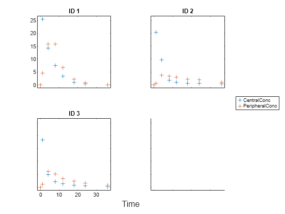
Display the data.
sbiotrellis(gData,"ID","Time",["CentralConc","PeripheralConc"],...
            Marker="+",LineStyle="none");
Use the built-in PK library to construct a two-compartment model with infusion dosing and first-order elimination. Use the configset object to turn on unit conversion.
pkmd                 = PKModelDesign;
pkc1                 = addCompartment(pkmd,"Central");
pkc1.DosingType      = "Infusion";
pkc1.EliminationType = "linear-clearance";
pkc1.HasResponseVariable = true;
pkc2                 = addCompartment(pkmd,"Peripheral");
model2cpt            = construct(pkmd);
configset            = getconfigset(model2cpt);
configset.CompileOptions.UnitConversion = true;
Assume every individual receives an infusion dose at time = 0, with a total infusion amount of 100 mg at a rate of 50 mg/hour. For details on setting up different dosing strategies, see Doses in SimBiology Models.
dose             = sbiodose("dose","TargetName","Drug_Central");
dose.StartTime   = 0;
dose.Amount      = 100;
dose.Rate        = 50;
dose.AmountUnits = "milligram";
dose.TimeUnits   = "hour";
dose.RateUnits   = "milligram/hour";
Create a problem object.
problem = fitproblem
problem =
  fitproblem with properties:

   Required:
                   Data: [0×0 groupedData]
              Estimated: [1×0 estimatedInfo]
            FitFunction: "sbiofit"
                  Model: [0×0 SimBiology.Model]
            ResponseMap: [1×0 string]

   Optional:
                  Doses: [0×0 SimBiology.Dose]
           FunctionName: "auto"
                Options: []
           ProgressPlot: 0
            UseParallel: 0
               Variants: [0×0 SimBiology.Variant]
             ErrorModel: "constant"

   sbiofit options:
                 Pooled: "auto"
    SensitivityAnalysis: "auto"
                Weights: []
Define the required properties of the object.
problem.Data        = gData;
problem.Estimated   = estimatedInfo(["log(Central)","log(Peripheral)","Q12","Cl_Central"],InitialValue=[1 1 1 1]);
problem.Model       = model2cpt;
problem.ResponseMap = ["Drug_Central = CentralConc","Drug_Peripheral = PeripheralConc"];
Define the dose to be applied during fitting.
problem.Doses = dose;
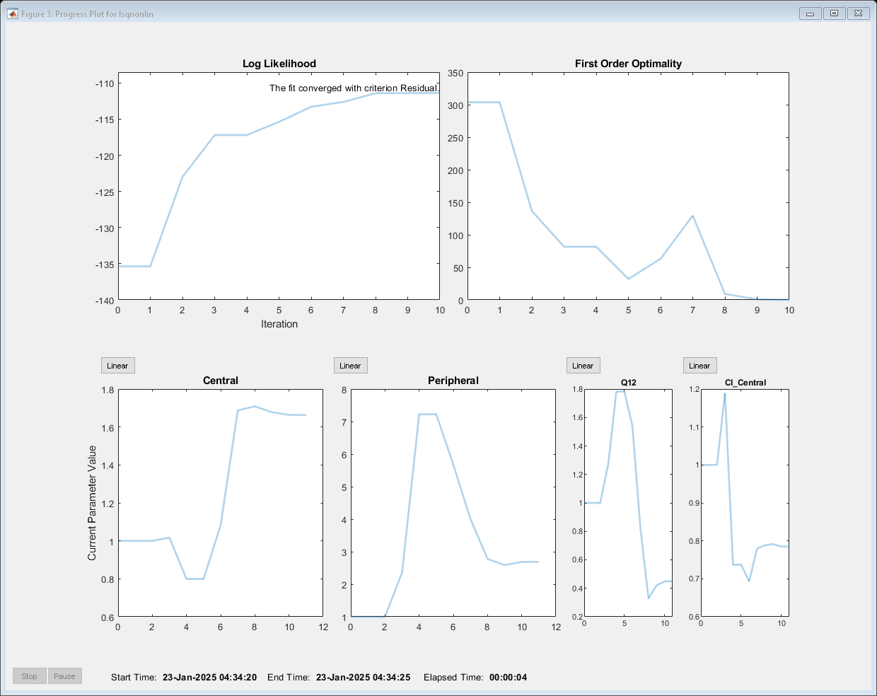
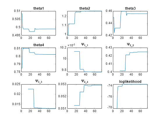
Show the progress of the estimation.
problem.ProgressPlot = true;
Fit the model to all of the data pooled together: that is, estimate one set of parameters for all individuals by setting the Pooled property to true.
problem.Pooled = true;
Perform the estimation using the fit function of the object.
pooledFit = fit(problem);
Display the estimated parameter values.
pooledFit.ParameterEstimates
ans=4×3 table
         Name         Estimate    StandardError
    ______________    ________    _____________

    {'Central'   }     1.6627        0.16569
    {'Peripheral'}     2.6864         1.0644
    {'Q12'       }    0.44945        0.19943
    {'Cl_Central'}    0.78497       0.095621
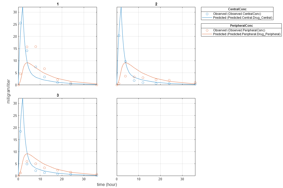
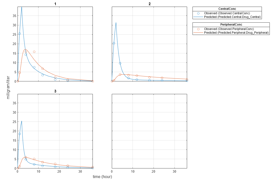
Plot the fitted results.
plot(pooledFit);
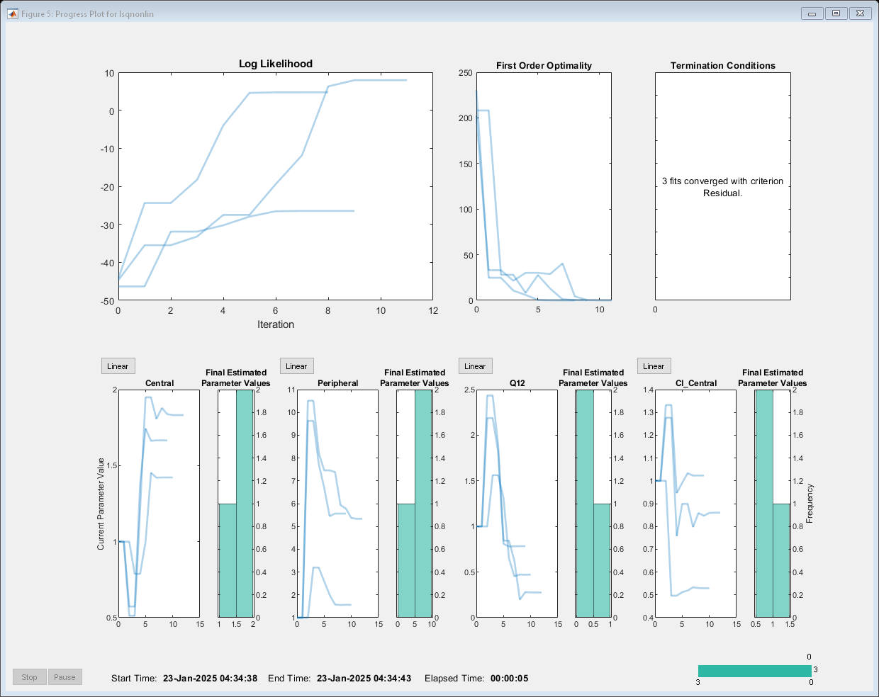
Estimate one set of parameters for each individual and see if the parameter estimates improve.
problem.Pooled  = false;
unpooledFit     = fit(problem);
Display the estimated parameter values.
unpooledFit.ParameterEstimates
ans=4×3 table
         Name         Estimate    StandardError
    ______________    ________    _____________

    {'Central'   }      1.422        0.12334
    {'Peripheral'}     1.5619        0.36355
    {'Q12'       }    0.47163        0.15196
    {'Cl_Central'}     0.5291       0.036978
ans=4×3 table
         Name         Estimate    StandardError
    ______________    ________    _____________

    {'Central'   }     1.8322       0.019672
    {'Peripheral'}     5.3364        0.65327
    {'Q12'       }     0.2764       0.030799
    {'Cl_Central'}    0.86035       0.026257
ans=4×3 table
         Name         Estimate    StandardError
    ______________    ________    _____________

    {'Central'   }     1.6657       0.038529
    {'Peripheral'}     5.5632        0.37063
    {'Q12'       }    0.78361       0.058657
    {'Cl_Central'}     1.0233       0.027311
plot(unpooledFit);
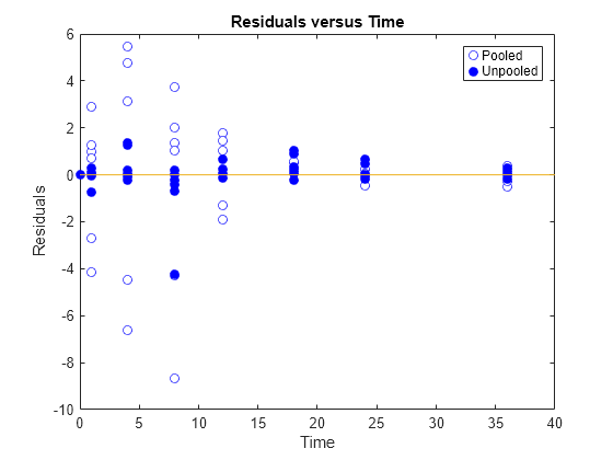
Generate a plot of the residuals over time to compare the pooled and unpooled fit results. The figure indicates unpooled fit residuals are smaller than those of the pooled fit, as expected. In addition to comparing residuals, other rigorous criteria can be used to compare the fitted results.
t = [gData.Time;gData.Time];
res_pooled = vertcat(pooledFit.R);
res_pooled = res_pooled(:);
res_unpooled = vertcat(unpooledFit.R);
res_unpooled = res_unpooled(:);
figure;
plot(t,res_pooled,"o",MarkerFaceColor="w",markerEdgeColor="b")
hold on
plot(t,res_unpooled,"o",MarkerFaceColor="b",markerEdgeColor="b")
refl = refline(0,0); % A reference line representing a zero residual
title("Residuals versus Time");
xlabel("Time");
ylabel("Residuals");
legend(["Pooled","Unpooled"]);
As illustrated, the unpooled fit accounts for variations due to the specific subjects in the study, and, in this case, the model fits better to the data. However, the pooled fit returns population-wide parameters. As an alternative, if you want to estimate population-wide parameters while considering individual variations, you can perform nonlinear mixed-effects (NLME) estimation by setting problem.FitFunction to sbiofitmixed.
problem.FitFunction = "sbiofitmixed";NLMEResults = fit(problem);
Display the estimated parameter values.
NLMEResults.IndividualParameterEstimates
ans=12×3 table
    Group         Name         Estimate
    _____    ______________    ________

      1      {'Central'   }     1.4623
      1      {'Peripheral'}     1.5306
      1      {'Q12'       }     0.4587
      1      {'Cl_Central'}    0.53208
      2      {'Central'   }      1.783
      2      {'Peripheral'}     6.6623
      2      {'Q12'       }     0.3589
      2      {'Cl_Central'}     0.8039
      3      {'Central'   }     1.7135
      3      {'Peripheral'}     4.2844
      3      {'Q12'       }    0.54895
      3      {'Cl_Central'}     1.0708
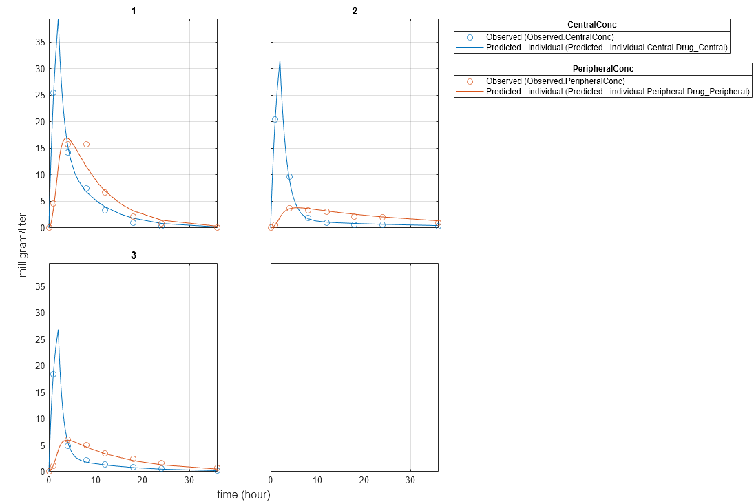
Plot the fitted results.
plot(NLMEResults);
Plot the conditional weighted residuals (CWRES) and individual weighted residuals (IWRES) of model predicted values.
plotResiduals(NLMEResults,'predictions')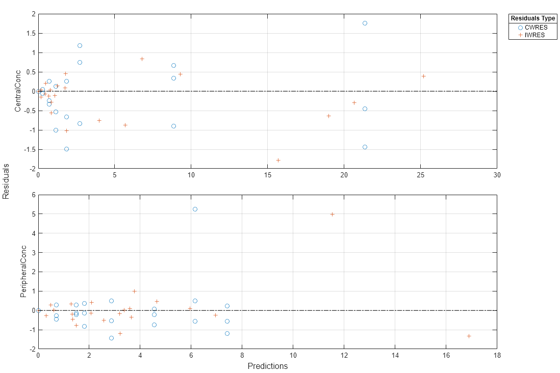
Import data to use for fitting. It comprises 12 groups of measurements across three responses: Drug, Target, and Complex. The Drug response includes measurements for all 12 groups, whereas the Target and Complex responses have measurements for only 8 and 4 groups, respectively. A group could represent a patient or an experimental or biological condition. Ndrug, Ntarget, and Ncomplex columns represent the constant number of groups that have the measurements for the corresponding responses. Each group has its own dosing amount, represented by the Dose column.
dataTMDD = readtable('tmddData_final.csv');Display the first few rows of the data set.
head(dataTMDD)
    ID    Time    Dose      Drug       Target    Complex    Ndrug    Ntarget    Ncomplex
    __    ____    ____    _________    ______    _______    _____    _______    ________

    1       0      10           NaN       NaN        NaN     12         8          4
    1     0.5     NaN        1.2131    10.116    0.36602     12         8          4
    1       1     NaN       0.74803    9.4694    0.61803     12         8          4
    1       2     NaN       0.28601    9.2434    0.84304     12         8          4
    1       4     NaN      0.048002    9.6184    0.83204     12         8          4
    1       8     NaN     0.0080003    9.6334    0.67203     12         8          4
    1      12     NaN     0.0060003    9.4574    0.54002     12         8          4
    1      16     NaN     0.0050002    9.7914    0.40502     12         8          4
Convert the data to a groupedData format.
gData = groupedData(dataTMDD);
gData.Properties.VariableUnits = ["","hour","nanomole","nanomole/liter","nanomole/liter","nanomole/liter","","",""];
gData.Properties.GroupVariableName = "ID";
gData.Properties.IndependentVariableName = "Time";
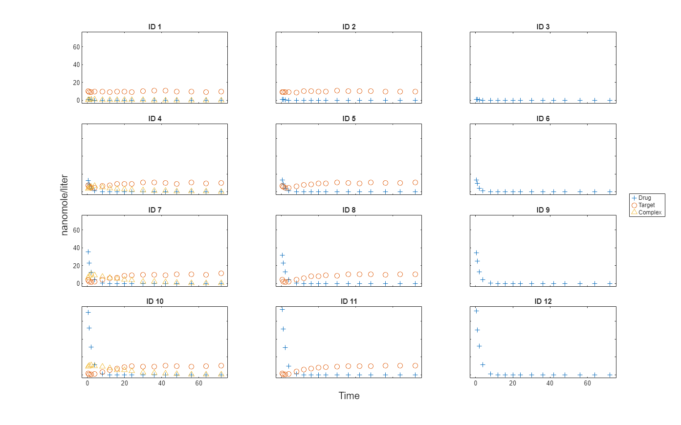
Plot the responses: Drug, Target, and Complex.
t = sbiotrellis(gData,"ID","Time","Drug",Marker="+",LineStyle="none");
plot(t,gData,"ID","Time","Target",Marker="o",LineStyle="none");
plot(t,gData,"ID","Time","Complex",Marker="^",LineStyle="none");
t.hFig.Position = [100 100 1280 800];
t.YLabel = "nanomole/liter";
Load the target-mediated drug deposition (TMDD) model. For details about the model, see Scan Dosing Regimens Using SimBiology Model Analyzer App.
sbioloadproject("tmdd_with_TO.sbproj","m1");
The data has 12 groups of measurements, and each group has its own dose amount. Create a corresponding dose object for each group using the dosing information from the data. During the subsequent fitting step, the fit function applies each dose to each group in the same order that the groups appear in the input data. For details on setting up doses, see dosing.
dose = sbiodose("Dose");
dose.TargetName = "Plasma.Drug";
doses = createDoses(gData,"Dose","",dose);
Specify parameters to estimate and their initial values. Also set upper and lower parameter bounds.
paramsToEstimate = estimatedInfo(["log(km)","log(kon)","log(koff)"],InitialValue=0.01,Bounds=[1e-05 1]);
Map the measurement data to the corresponding model components.
responseMap = ["Plasma.Drug = Drug",...
               "Plasma.Target = Target",...
               "Plasma.Complex = Complex"];
Define the algorithm options.
options                     = optimoptions("lsqnonlin");
options.StepTolerance       = 1e-08;
options.FunctionTolerance   = 1e-08;
options.OptimalityTolerance = 1e-06;
options.MaxIterations       = 100;
Define the fit problem.
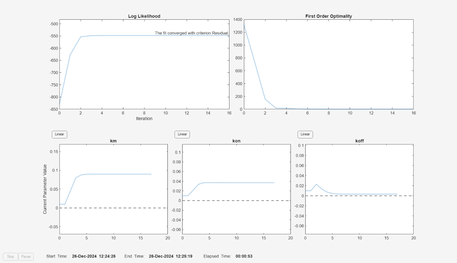
f              = fitproblem(FitFunction="sbiofit");
f.Data         = gData;
f.Estimated    = paramsToEstimate;
f.Model        = m1;
f.ResponseMap  = responseMap;

f.Doses        = doses;
f.FunctionName = "lsqnonlin";
f.Options      = options;
f.Pooled       = true;
f.ProgressPlot = true;
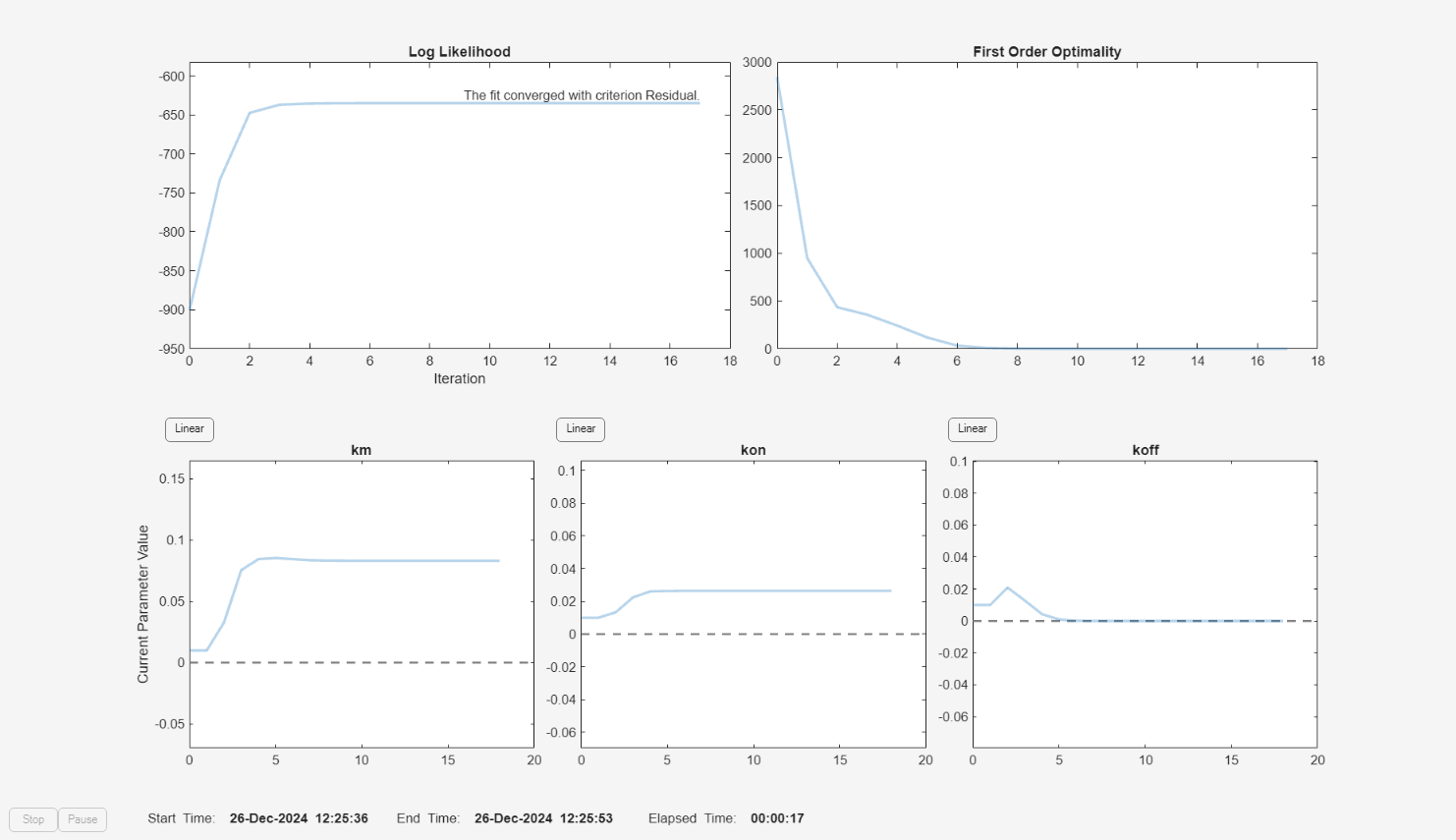
Run the fit with weights set to 1.
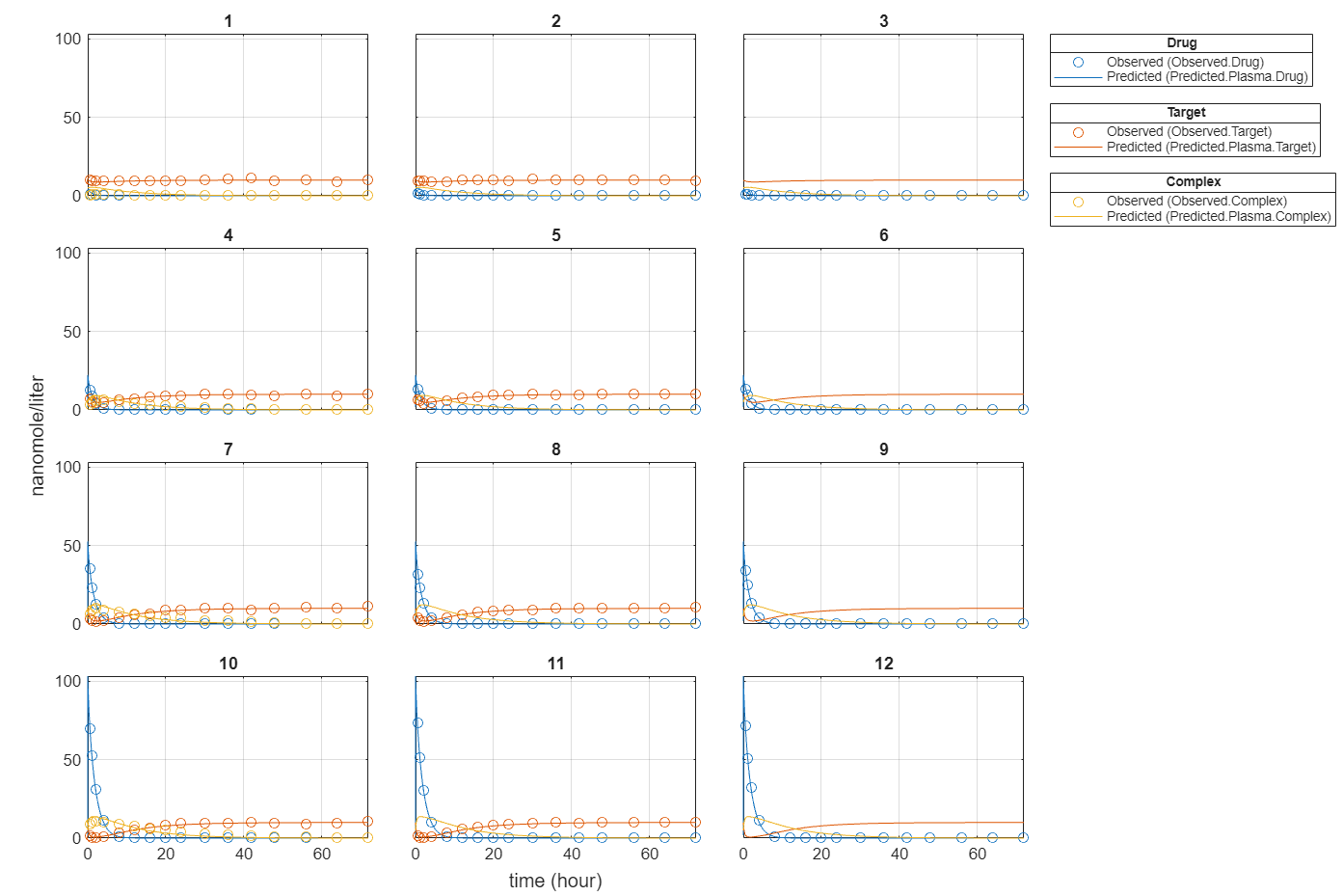
f.Weights = [ones(size(gData.Drug)) ones(size(gData.Target)) ones(size(gData.Complex))];
fitEqualWeights = fit(f);
plot(fitEqualWeights);
Plot all groups in one plot for each response.
plot(fitEqualWeights,PlotStyle="one axes");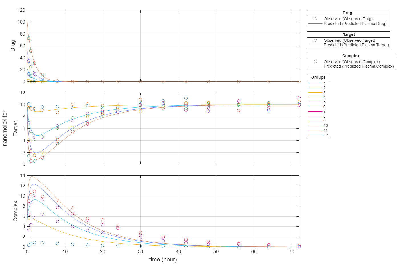
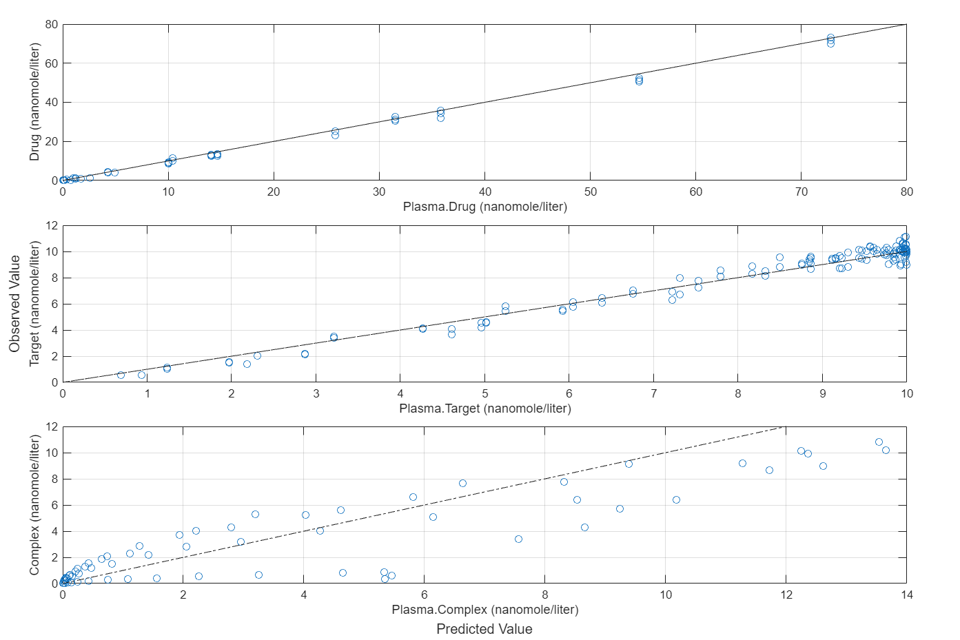
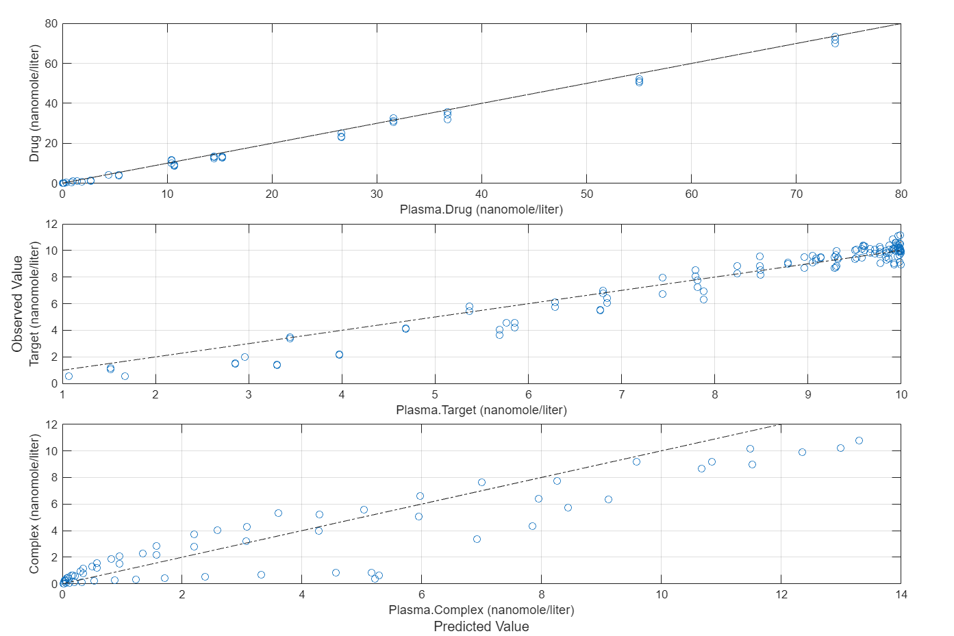
Compare the predictions to the actual data.
plotActualVersusPredicted(fitEqualWeights)
In this data set, the response Drug has 12 groups of measurements, Target has 8 groups of measurements, and Complex has 4 groups of measurements. The varying number of measurements among these responses might stem from the experimental design. To address these differences, you might consider experimenting with weights that are inversely proportional to the number of measurement groups.
f.Weights = [1./gData.Ndrug 1./gData.Ntarget 1./gData.Ncomplex];
fitInverseWeights = fit(f);
plot(fitInverseWeights);
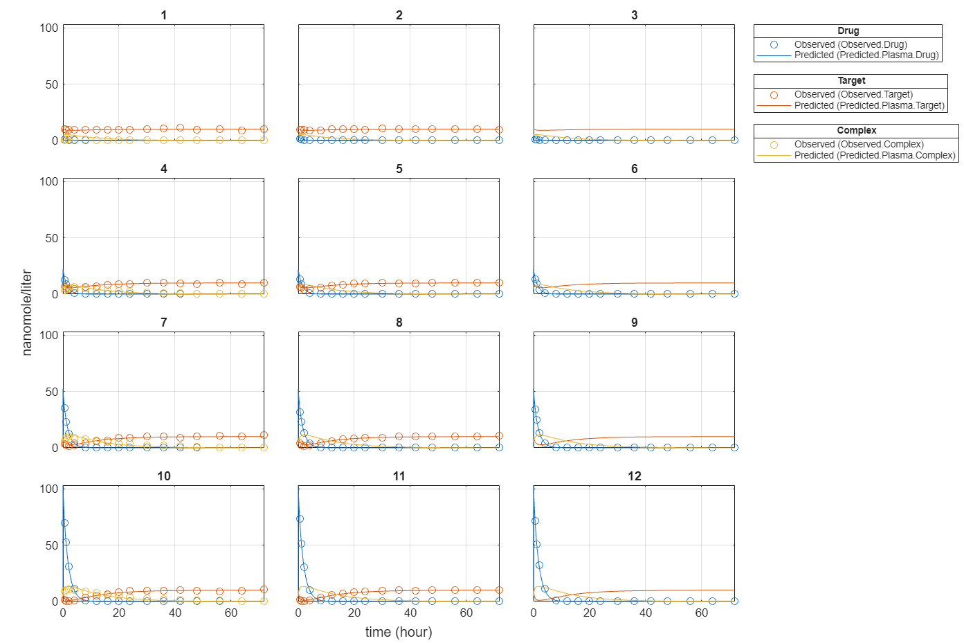
Plot all groups in one plot for each response.
plot(fitInverseWeights,PlotStyle="one axes");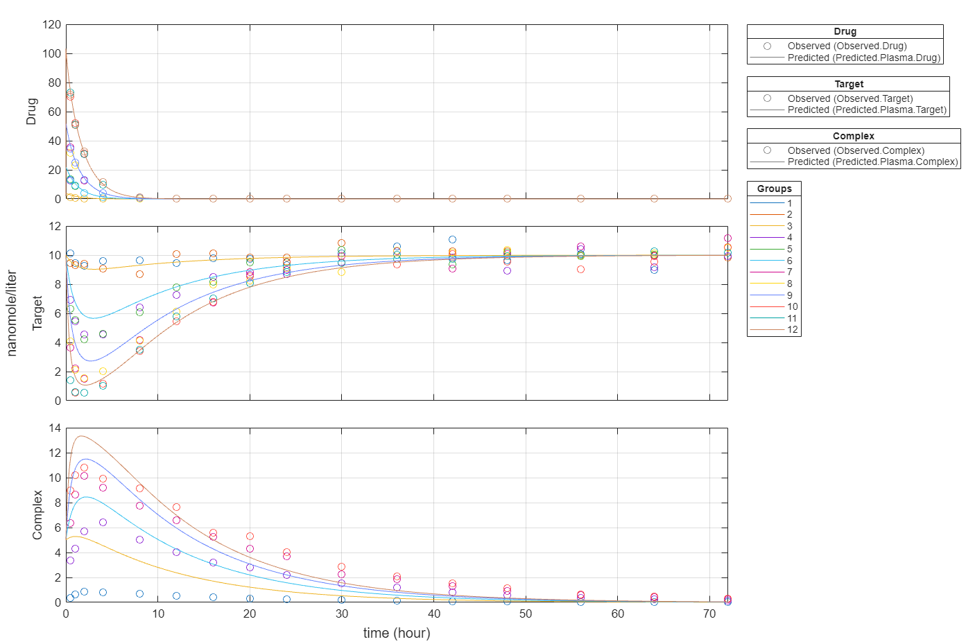
Compare the predictions to the actual data.
plotActualVersusPredicted(fitInverseWeights)
More About
Version History
Introduced in R2021b
See Also
sbiofit | sbiofitmixed | EstimatedInfo object | groupedData object | LeastSquaresResults object | NLINResults object | OptimResults object | sbiofitmixed | nlinfit (Statistics and Machine Learning Toolbox) | fmincon (Optimization Toolbox) | fminunc (Optimization Toolbox) | fminsearch | lsqcurvefit (Optimization Toolbox) | lsqnonlin (Optimization Toolbox) | patternsearch (Global Optimization Toolbox) | ga (Global Optimization Toolbox) | particleswarm (Global Optimization Toolbox)