Automated Feature Engineering for Regression

The genrfeatures function enables you to automate the feature engineering process in the context of a machine learning workflow. Before passing tabular training data to a regression model, you can create new features from the predictors in the data by using genrfeatures. Use the returned data to train the model.

Generate new features based on your machine learning workflow.

• To generate features for an interpretable regression model, use the default TargetLearner value of "linear" in the call to genrfeatures. You can then use the returned data to train a linear regression model. For an example, see Interpret Linear Model with Generated Features.

• To generate features that can lead to better model prediction, specify TargetLearner="bag" or TargetLearner="gaussian-svm" in the call to genrfeatures. You can then use the returned data to train a bagged ensemble regression model or a support vector machine (SVM) regression model with a Gaussian kernel, respectively. For an example, see Generate New Features to Improve Bagged Ensemble Performance.

To better understand the generated features, use the describe function of the FeatureTransformer object. To apply the same training set feature transformations to a test or validation set, use the transform function of the FeatureTransformer object.

Interpret Linear Model with Generated Features

Use automated feature engineering to generate new features. Train a linear regression model using the generated features. Interpret the relationship between the generated features and the trained model.

Load the patients data set. Create a table from a subset of the variables. Display the first few rows of the table.

load patients
Tbl = table(Age,Diastolic,Gender,Height,SelfAssessedHealthStatus, ...
    Smoker,Weight,Systolic);
head(Tbl)

    Age    Diastolic      Gender      Height    SelfAssessedHealthStatus    Smoker    Weight    Systolic
    ___    _________    __________    ______    ________________________    ______    ______    ________

    38        93        {'Male'  }      71           {'Excellent'}          true       176        124   
    43        77        {'Male'  }      69           {'Fair'     }          false      163        109   
    38        83        {'Female'}      64           {'Good'     }          false      131        125   
    40        75        {'Female'}      67           {'Fair'     }          false      133        117   
    49        80        {'Female'}      64           {'Good'     }          false      119        122   
    46        70        {'Female'}      68           {'Good'     }          false      142        121   
    33        88        {'Female'}      64           {'Good'     }          true       142        130   
    40        82        {'Male'  }      68           {'Good'     }          false      180        115   

Generate 10 new features from the variables in Tbl. Specify the Systolic variable as the response. By default, genrfeatures assumes that the new features will be used to train a linear regression model.

rng("default") % For reproducibility
[T,NewTbl] = genrfeatures(Tbl,"Systolic",10)

T = 
  FeatureTransformer with properties:

                     Type: 'regression'
            TargetLearner: 'linear'
    NumEngineeredFeatures: 10
      NumOriginalFeatures: 0
         TotalNumFeatures: 10

NewTbl=100×11 table
    zsc(d(Smoker))    q8(Age)    eb8(Age)    zsc(sin(Height))    zsc(kmd8)    q6(Height)    eb8(Diastolic)    q8(Diastolic)    zsc(fenc(c(SelfAssessedHealthStatus)))    q10(Weight)    Systolic
    ______________    _______    ________    ________________    _________    __________    ______________    _____________    ______________________________________    ___________    ________

         1.3863          4          5              1.1483         -0.56842        6               8                 8                         0.27312                        7            124   
       -0.71414          6          6             -0.3877          -2.0772        5               2                 2                         -1.4682                        6            109   
       -0.71414          4          5              1.1036         -0.21519        2               4                 5                         0.82302                        3            125   
       -0.71414          5          6             -1.4552         -0.32389        4               2                 2                         -1.4682                        4            117   
       -0.71414          8          8              1.1036           1.2302        2               3                 4                         0.82302                        1            122   
       -0.71414          7          7             -1.5163         -0.88497        4               1                 1                         0.82302                        5            121   
         1.3863          3          3              1.1036          -1.1434        2               6                 6                         0.82302                        5            130   
       -0.71414          5          6             -1.5163          -0.3907        4               4                 5                         0.82302                        8            115   
       -0.71414          1          2             -1.5163           0.4278        4               3                 3                         0.27312                        9            115   
       -0.71414          2          3            -0.26055        -0.092621        3               5                 6                         0.27312                        3            118   
       -0.71414          7          7             -1.5163          0.16737        4               2                 2                         0.27312                        2            114   
       -0.71414          6          6            -0.26055         -0.32104        3               1                 1                         -1.8348                        5            115   
       -0.71414          1          1              1.1483        -0.051074        6               1                 1                         -1.8348                        7            127   
         1.3863          5          5             0.14351           2.3695        6               8                 8                         0.27312                        10           130   
       -0.71414          3          4             0.96929         0.092962        2               3                 4                         0.82302                        3            114   
         1.3863          8          8              1.1483        -0.049336        6               7                 8                         0.82302                        8            130   
      ⋮

T is a FeatureTransformer object that can be used to transform new data, and newTbl contains the new features generated from the Tbl data.

To better understand the generated features, use the describe object function of the FeatureTransformer object. For example, inspect the first two generated features.

describe(T,1:2)

                         Type        IsOriginal    InputVariables                          Transformations
                      ___________    __________    ______________    ___________________________________________________________

    zsc(d(Smoker))    Numeric          false           Smoker        Variable of type double converted from an integer data type
                                                                     Standardization with z-score (mean = 0.34, std = 0.4761)
    q8(Age)           Categorical      false           Age           Equiprobable binning (number of bins = 8)

The first feature in newTbl is a numeric variable, created by first converting the values of the Smoker variable to a numeric variable of type double and then transforming the results to z-scores. The second feature in newTbl is a categorical variable, created by binning the values of the Age variable into 8 equiprobable bins.

Use the generated features to fit a linear regression model without any regularization.

Mdl = fitrlinear(NewTbl,"Systolic",Lambda=0);

Plot the coefficients of the predictors used to train Mdl. Note that fitrlinear expands categorical predictors before fitting a model.

p = length(Mdl.Beta);
[sortedCoefs,expandedIndex] = sort(Mdl.Beta,ComparisonMethod="abs");
sortedExpandedPreds = Mdl.ExpandedPredictorNames(expandedIndex);
bar(sortedCoefs,Horizontal="on")
yticks(1:2:p)
yticklabels(sortedExpandedPreds(1:2:end))
xlabel("Coefficient")
ylabel("Expanded Predictors")
title("Coefficients for Expanded Predictors")

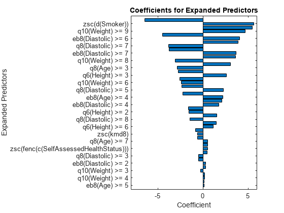
Identify the predictors whose coefficients have larger absolute values.

bigCoefs = abs(sortedCoefs) >= 4;
flip(sortedExpandedPreds(bigCoefs))

ans = 1x6 cell
    {'eb8(Diastolic) >= 5'}    {'zsc(d(Smoker))'}    {'q8(Age) >= 2'}    {'q10(Weight) >= 9'}    {'q6(Height) >= 5'}    {'eb8(Diastolic) >= 6'}

You can use partial dependence plots to analyze the categorical features whose levels have large coefficients in terms of absolute value. For example, inspect the partial dependence plot for the eb8(Diastolic) variable, whose levels eb8(Diastolic) >= 5 and eb8(Diastolic) >= 6 have coefficients with large absolute values. These two levels correspond to noticeable changes in the predicted Systolic values.

plotPartialDependence(Mdl,"eb8(Diastolic)",NewTbl);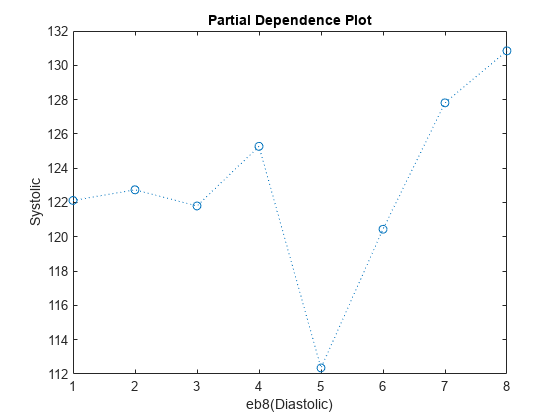

Generate New Features to Improve Bagged Ensemble Performance

Use genrfeatures to engineer new features before training a bagged ensemble regression model. Before making predictions on new data, apply the same feature transformations to the new data set. Compare the test set performance of the ensemble that uses the engineered features to the test set performance of the ensemble that uses the original features.

Read power outage data into the workspace as a table. Remove observations with missing values, and display the first few rows of the table.

outages = readtable("outages.csv");
Tbl = rmmissing(outages);
head(Tbl)

       Region           OutageTime        Loss     Customers     RestorationTime            Cause       
    _____________    ________________    ______    __________    ________________    ___________________

    {'SouthWest'}    2002-02-01 12:18    458.98    1.8202e+06    2002-02-07 16:50    {'winter storm'   }
    {'SouthEast'}    2003-02-07 21:15     289.4    1.4294e+05    2003-02-17 08:14    {'winter storm'   }
    {'West'     }    2004-04-06 05:44    434.81    3.4037e+05    2004-04-06 06:10    {'equipment fault'}
    {'MidWest'  }    2002-03-16 06:18    186.44    2.1275e+05    2002-03-18 23:23    {'severe storm'   }
    {'West'     }    2003-06-18 02:49         0             0    2003-06-18 10:54    {'attack'         }
    {'NorthEast'}    2003-07-16 16:23    239.93         49434    2003-07-17 01:12    {'fire'           }
    {'MidWest'  }    2004-09-27 11:09    286.72         66104    2004-09-27 16:37    {'equipment fault'}
    {'SouthEast'}    2004-09-05 17:48    73.387         36073    2004-09-05 20:46    {'equipment fault'}

Some of the variables, such as OutageTime and RestorationTime, have data types that are not supported by regression model training functions like fitrensemble.

Partition the data into training and test sets. Use approximately 70% of the observations as training data, and 30% of the observations as test data. Partition the data using cvpartition.

rng("default") % For reproducibility of the partition
c = cvpartition(size(Tbl,1),Holdout=0.30);
TrainTbl = Tbl(training(c),:);
TestTbl = Tbl(test(c),:);

Use the training data to generate 30 new features to fit a bagged ensemble. By default, the 30 features include original features that can be used as predictors by a bagged ensemble.

[Transformer,NewTrainTbl] = genrfeatures(TrainTbl,"Loss",30, ...
    TargetLearner="bag");
Transformer

Transformer = 
  FeatureTransformer with properties:

                     Type: 'regression'
            TargetLearner: 'bag'
    NumEngineeredFeatures: 27
      NumOriginalFeatures: 3
         TotalNumFeatures: 30

Create NewTestTbl by applying the transformations stored in the object Transformer to the test data.

NewTestTbl = transform(Transformer,TestTbl);

Train a bagged ensemble using the original training set TrainTbl, and compute the mean squared error (MSE) of the model on the original test set TestTbl. Specify only the three predictor variables that can be used by fitrensemble (Region, Customers, and Cause), and omit the two datetime predictor variables (OutageTime and RestorationTime). Then, train a bagged ensemble using the transformed training set NewTrainTbl, and compute the MSE of the model on the transformed test set NewTestTbl.

originalMdl = fitrensemble(TrainTbl,"Loss ~ Region + Customers + Cause", ...
    Method="bag");
originalTestMSE = loss(originalMdl,TestTbl)

originalTestMSE = 
1.8999e+06

newMdl = fitrensemble(NewTrainTbl,"Loss",Method="bag");
newTestMSE = loss(newMdl,NewTestTbl)

newTestMSE = 
1.8617e+06

newTestMSE is less than originalTestMSE, which suggests that the bagged ensemble trained on the transformed data performs slightly better than the bagged ensemble trained on the original data.

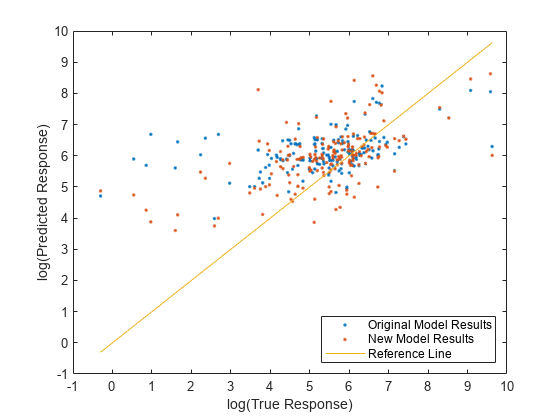
Compare the predicted test set response values to the true response values for both models. Plot the log of the predicted response along the vertical axis and the log of the true response (Loss) along the horizontal axis. Points on the reference line indicate correct predictions. A good model produces predictions that are scattered near the line.

predictedTestY = predict(originalMdl,TestTbl);
newPredictedTestY = predict(newMdl,NewTestTbl);

plot(log(TestTbl.Loss),log(predictedTestY),".")
hold on
plot(log(TestTbl.Loss),log(newPredictedTestY),".")
hold on
plot(log(TestTbl.Loss),log(TestTbl.Loss))
hold off
xlabel("log(True Response)")
ylabel("log(Predicted Response)")
legend(["Original Model Results","New Model Results","Reference Line"], ...
    Location="southeast")
xlim([-1 10])
ylim([-1 10])