dwt2
Single-level 2-D discrete wavelet transform
Syntax
Description
[
computes the single-level 2-D DWT with the extension mode
cA,cH,cV,cD] = dwt2(___,"mode",extmode)extmode. Include this argument after all other
arguments.
Note
For gpuArray inputs, the supported modes are
"symh" ("sym") and
"per". All "mode" options except
"per" are converted to "symh". See
the example Single-Level 2-D Discrete Wavelet Transform on a GPU.
Examples
Load and display an image.
load tartan
imagesc(X)
colormap(map)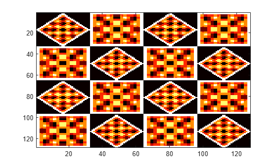
Obtain the single-level 2-D discrete wavelet transform of the image using the order 4 symlet and periodic extension.
[cA,cH,cV,cD] = dwt2(X,"sym4","mode","per");
Display the diagonal detail coefficients and the approximation coefficients.
imagesc(cD)
title("Diagonal Detail Coefficients")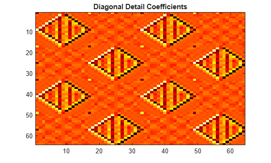
imagesc(cA)
title("Approximation Coefficients")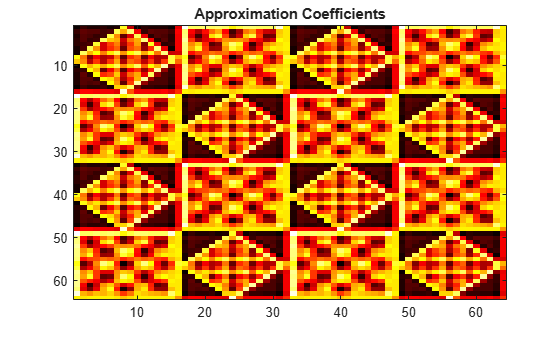
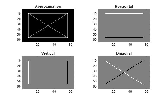
Load and display an image.
load xbox
imagesc(xbox)
colormap gray
Generate the lowpass and highpass decomposition filters for the Haar wavelet.
[LoD,HiD] = wfilters("haar","d");
Use the filters to perform a single-level 2-D wavelet decomposition. Use half-point symmetric extension. Display the approximation and detail coefficients.
[cA,cH,cV,cD] = dwt2(xbox,LoD,HiD,"mode","symh");
tiledlayout(2,2)
nexttile
imagesc(cA)
colormap gray
title("Approximation")
nexttile
imagesc(cH)
colormap gray
title("Horizontal")
nexttile
imagesc(cV)
colormap gray
title("Vertical")
nexttile
imagesc(cD)
colormap gray
title("Diagonal")
Refer to GPU Computing Requirements (Parallel Computing Toolbox) to see what GPUs are supported.
Load an image. Put the image on the GPU using gpuArray. Save the current extension mode.
load mask
imgg = gpuArray(X);
origMode = dwtmode("status","nodisp");
Use dwtmode to change the extension mode to zero-padding. Obtain the single-level 2-D DWT of the image on the GPU using the db2 wavelet.
dwtmode("zpd","nodisp")
[cA,cH,cV,cD] = dwt2(imgg,"db2");
The current extension mode zpd is not supported for gpuArray input. Therefore, the DWT is instead performed using the "sym" extension mode. Confirm this by taking the DWT of imgg with the extension mode set to "sym" and compare with the previous result.
[cAsym,cHsym,cVsym,cDsym] = dwt2(imgg,"db2","mode","sym");
[max(abs(cA(:)-cAsym(:))) max(abs(cH(:)-cHsym(:))) ...
    max(abs(cV(:)-cVsym(:))) max(abs(cD(:)-cDsym(:)))]
ans =

     0     0     0     0
An unsupported extension mode specified as an input argument is converted to "sym". Confirm that taking the DWT of imgg with "mode" set to an unsupported mode also defaults to the "sym" extension mode.
[cA,cH,cV,cD] = dwt2(imgg,"db2","mode","spd");
[max(abs(cA(:)-cAsym(:))) max(abs(cH(:)-cHsym(:))) ...
    max(abs(cV(:)-cVsym(:))) max(abs(cD(:)-cDsym(:)))]
ans =

     0     0     0     0
Change the current extension mode to periodic. Obtain the single-level DWT of the image on the GPU using the db2 wavelet.
dwtmode("per","nodisp")
[cA,cH,cV,cD] = dwt2(imgg,"db2");
Confirm the current extension mode "per" is supported for gpuArray input.
[cAper,cHper,cVper,cDper] = dwt2(imgg,"db2","mode","per");
[max(abs(cA(:)-cAper(:))) max(abs(cH(:)-cHper(:))) ...
    max(abs(cV(:)-cVper(:))) max(abs(cD(:)-cDper(:)))]
ans =

     0     0     0     0
Restore the extension mode to the original setting.
dwtmode(origMode,"nodisp")Input Arguments
Output Arguments
Algorithms
The 2-D wavelet decomposition algorithm for images is similar to the one-dimensional case. The two-dimensional wavelet and scaling functions are obtained by taking the tensor products of the one-dimensional wavelet and scaling functions. This kind of two-dimensional DWT leads to a decomposition of approximation coefficients at level j in four components: the approximation at level j + 1, and the details in three orientations (horizontal, vertical, and diagonal). The following chart describes the basic decomposition steps for images.

where
 — Downsample columns: keep the even-indexed columns
 — Downsample rows: keep the even-indexed rows
 — Convolve with filter X the rows of
the entry
— Convolve with filter X the rows of
the entry — Convolve with filter X the columns
of the entry
— Convolve with filter X the columns
of the entry
The decomposition is initialized by setting the approximation coefficients equal to the image s: cA0 = s.
Note
To deal with signal-end effects introduced by a convolution-based algorithm, the
1-D and 2-D DWT use a global variable managed by dwtmode. This variable defines
the kind of signal extension mode used. The possible options include zero-padding
and symmetric extension, which is the default mode.
References
[1] Daubechies, Ingrid. Ten Lectures on Wavelets. CBMS-NSF Regional Conference Series in Applied Mathematics 61. Philadelphia, Pa: Society for Industrial and Applied Mathematics, 1992.
[2] Mallat, S.G. “A Theory for Multiresolution Signal Decomposition: The Wavelet Representation.” IEEE Transactions on Pattern Analysis and Machine Intelligence 11, no. 7 (July 1989): 674–93. https://doi.org/10.1109/34.192463.
[3] Meyer, Y. Wavelets and Operators. Translated by D. H. Salinger. Cambridge, UK: Cambridge University Press, 1995.