balreal

Gramian-based input/output balancing of state-space realizations

Syntax

[sysb,g] = balreal(sys) [sysb,g,T,Ti] = balreal(sys) [___] = balreal(sys,opts)

Description

[sysb,g] = balreal(sys) computes a balanced realization sysb for the stable portion of the LTI model sys. balreal handles both continuous and discrete systems. If sys is not a state-space model, it is first and automatically converted to state space using ss.

For stable systems, sysb is an equivalent realization for which the controllability and observability Gramians are equal and diagonal, their diagonal entries forming the vector g of Hankel singular values. Small entries in g indicate states that can be removed to simplify the model (use modred to reduce the model order).

If sys has unstable poles, its stable part is isolated, balanced, and added back to its unstable part to form sysb. The entries of g corresponding to unstable modes are set to Inf.

[sysb,g,T,Ti] = balreal(sys) also returns the vector g containing the diagonal of the balanced Gramian, the state similarity transformation x_b = Tx used to convert sys to sysb, and the inverse transformation Ti = T^-1.

If the system is normalized properly, the diagonal g of the joint Gramian can be used to reduce the model order. Because g reflects the combined controllability and observability of individual states of the balanced model, you can delete those states with a small g(i) while retaining the most important input-output characteristics of the original system. Use modred to perform the state elimination.

[___] = balreal(sys,opts) computes the balanced realization using options that you specify using balredOptions. Options include offset and tolerance options for computing the stable-unstable decompositions. The options also allow you to limit the Gramian computation to particular time and frequency intervals. See balredOptions for details.

Examples

collapse all

Balanced Realization of Stable System

Open Live Script

Consider the following zero-pole-gain model, with near-canceling pole-zero pairs:

sys = zpk([-10 -20.01],[-5 -9.9 -20.1],1)

sys =
 
     (s+10) (s+20.01)
  ----------------------
  (s+5) (s+9.9) (s+20.1)
 
Continuous-time zero/pole/gain model.

A state-space realization with balanced gramians is obtained by

[sysb,g] = balreal(sys);

The diagonal entries of the joint gramian are

g'

ans = 1×3

    0.1006    0.0001    0.0000

This indicates that the last two states of sysb are weakly coupled to the input and output. You can then delete these states by

sysr = modred(sysb,[2 3],'del');

This yields the following first-order approximation of the original system.

zpk(sysr)

ans =
 
   1.0001
  --------
  (s+4.97)
 
Continuous-time zero/pole/gain model.

Compare the Bode responses of the original and reduced-order models.

bodeplot(sys,sysr,'r--')

Figure contains 2 axes objects. Axes object 1 with ylabel Magnitude (dB) contains 2 objects of type line. These objects represent sys, sysr. Axes object 2 with ylabel Phase (deg) contains 2 objects of type line. These objects represent sys, sysr.

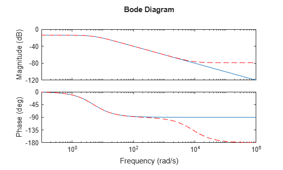
The plots shows that removing the second and third states does not have much effect on system dynamics.

Balanced Realization of Unstable System

Open Live Script

Create an unstable system.

sys = tf(1,[1 0 -1])

sys =
 
     1
  -------
  s^2 - 1
 
Continuous-time transfer function.

Apply balreal to create a balanced-gramian realization.

[sysbal,g] = balreal(sys)

sysbal =
 
  A = 
       x1  x2
   x1   1   0
   x2   0  -1
 
  B = 
            u1
   x1  -0.7071
   x2  -0.7071
 
  C = 
            x1       x2
   y1  -0.7071   0.7071
 
  D = 
       u1
   y1   0
 
Continuous-time state-space model.

g = 2×1

       Inf
    0.2500

The unstable pole shows up as Inf in the vector g.

Algorithms

Consider the model

$\begin{array}{l} \dot{x} = A x + B u \\ y = C x + D u \end{array}$

with controllability and observability Gramians W_c and W_o. The state coordinate transformation $\bar{x} = T x$ produces the equivalent model

$\begin{array}{l} \dot{\bar{x}} = T A T^{- 1} \bar{x} + T B u \\ y = C T^{- 1} \bar{x} + D u \end{array}$

and transforms the Gramians to

$\begin{matrix} {\bar{W}}_{c} = T W_{c} T^{T}, & {\bar{W}}_{o} = T^{- T} W_{o} \end{matrix} T^{- 1}$

The function balreal computes a particular similarity transformation T such that

${\bar{W}}_{c} = {\bar{W}}_{o} = d i a g (g)$

See [1], [2] for details on the algorithm.

If you use the TimeIntervals or FreqIntervals options of balredOptions, then balreal bases the balanced realization on time-limited or frequency-limited controllability and observability Gramians. For information about calculating time-limited and frequency-limited Gramians, see gram and [4].

References

[1] Laub, A.J., M.T. Heath, C.C. Paige, and R.C. Ward, "Computation of System Balancing Transformations and Other Applications of Simultaneous Diagonalization Algorithms," IEEE^® Trans. Automatic Control, AC-32 (1987), pp. 115-122.

[2] Moore, B., "Principal Component Analysis in Linear Systems: Controllability, Observability, and Model Reduction," IEEE Transactions on Automatic Control, AC-26 (1981), pp. 17-31.

[3] Laub, A.J., "Computation of Balancing Transformations," Proc. ACC, San Francisco, Vol.1, paper FA8-E, 1980.

[4] Gawronski, W. and J.N. Juang. “Model Reduction in Limited Time and Frequency Intervals.” International Journal of Systems Science. Vol. 21, Number 2, 1990, pp. 349–376.

Version History

Introduced before R2006a

References

[1] Laub, A., M. Heath, C. Paige, and R. Ward. “Computation of System Balancing Transformations and Other Applications of Simultaneous Diagonalization Algorithms.” IEEE Transactions on Automatic Control 32, no. 2 (February 1987): 115–22. https://doi.org/10.1109/TAC.1987.1104549.