getrom

Obtain reduced-order models when using zero-pole truncation method

Since R2025a

Syntax

rsys = getrom(R)

rsys = getrom(R,RollOff=Slope)

Description

rsys = getrom(R) returns a zero-pole-gain approximation of the original sparse model based on the specified R.Options.Focus and R.Options.MaxNumber options. rsys typically has far fewer states or degrees of freedom than the original sparse model.

rsys = getrom(R,RollOff=Slope) specifies the minimum roll-off slope Slope.

Examples

Reduce Sparse Beam Model Using Zero-Pole Truncation

This example shows how to obtain a reduced-order model of a structural beam using the zero-pole truncation method. For this example, consider a SISO sparse state-space model of a cantilever beam. This example uses the linearized model from the Linear Analysis of Cantilever Beam example.

Load the beam model.

load linBeam.mat
size(sys)

Sparse second-order model with 1 outputs, 1 inputs, and 3303 degrees of freedom.

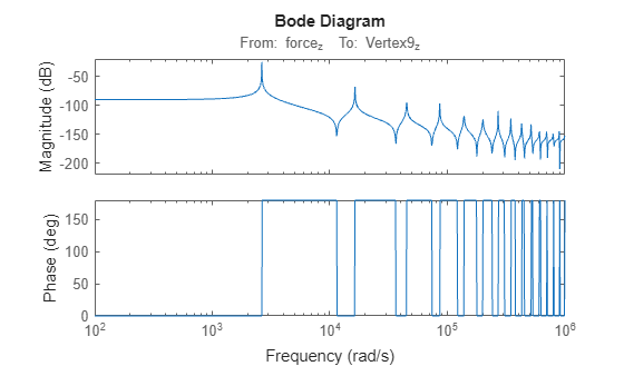
Analyze the frequency response of the model.

bodeplot(sys,w)

To perform sparse zero-pole truncation, first create a model order reduction task using reducespec with the "zpk" method.

R = reducespec(sys,"zpk");

For this task, set the frequency range of focus to compute modes up to 3e5 rad/s. Doing so prevents the algorithm from computing all the poles and zeros of the sparse model, which can take a long time in some cases.

R.Options.Focus = [0 3e5];
R.Options.Display = "off";

Run the model reduction algorithm. This computes the derived information, which are the poles, zeros, and gains of model, stored in the object R .

R = process(R);

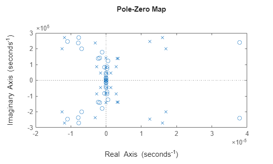
You can visualize the map of computed poles and zeros using the view function.

view(R)

Obtain the reduced zero-pole-gain approximation based on the specified frequency of focus.

rsys = getrom(R);
order(rsys)

ans = 
38

Compare the response of the original and reduced models.

figure;
opt = bodeoptions;
opt.PhaseWrapping = "on";
bodeplot(sys,rsys,"--",w,opt);

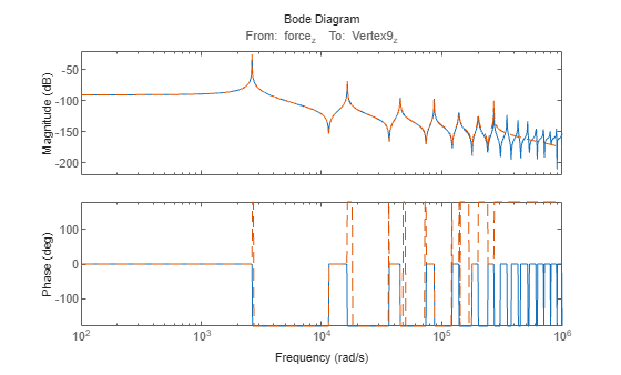
The reduced-order model provides a good approximation for the original sparse model in the specified range of interest.

Zero-Pole Truncation of Thermal Model

This example shows how to obtain a reduced model using zero-pole truncation of a sparse state-space model. This example uses a sparse model obtained from linearizing a thermal model of heat distribution in a circular cylindrical rod.

Load the model data.

load cylindricalRod.mat
sys = sparss(A,B,C,D,E);
w = logspace(-7,-1,20);
size(sys)

Sparse state-space model with 3 outputs, 1 inputs, and 7522 states.

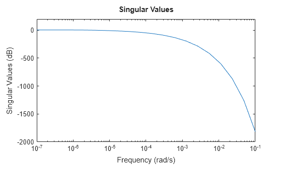
Analyze the frequency response of the model.

sigmaplot(sys,w)

Create a zero-pole truncation specification object for sys and specify the frequency band of focus. For this model, you can use a frequency range from 0 rad/s to 0.01 rad/s to obtain the low-order approximation.

R = reducespec(sys,"zpk");
R.Options.Focus = [0 1e-2];
R.Options.Display = "off";

Run the model reduction algorithm and obtain the reduced model.

R = process(R);
rsys = getrom(R);
sigmaplot(sys,rsys,w)

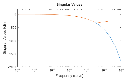
This thermal model has a very steep roll-off beyond 0.001 rad/s. By default, the reduced model obtained using getrom does not provide a good match for this roll-off. To mitigate this, you can use the RollOff argument of getrom and specify a minimum roll-off value beyond the frequency band of focus. Specify a roll-off slope value of -45, which corresponds to a rate of at least –900 db/decade.

rsys2 = getrom(R,RollOff=-45);
sigmaplot(sys,rsys2,w)

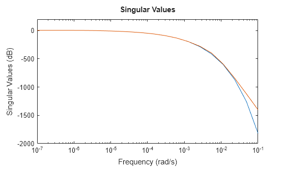
The reduced model now provides a much better approximation of the roll-off value.

Input Arguments

R — Model order reduction specification object

SparseZeroPoleTruncation object

Model order reduction specification object created using reducespec, specified as a SparseZeroPoleTruncation object.

Slope — Roll-off slope

nonpositive scalar | matrix

Roll-off slope, specified as a nonpositive scalar or matrix.

• Use a scalar value for SISO models or when the slope is uniform for all input-output pairs for MIMO models.

• Use a matrix when the slope is different for each input-output pair for MIMO models.

For example, Slope of -2 ensures the gain rolls off at a rate of at least –40 dB/decade (the roll-off rate of 1/s²).

Output Arguments

rsys — Reduced-order model

zpk model

Reduced-order model, returned as a zero-pole-gain (zpk) model.

Version History

Introduced in R2025a