poctave
Generate octave spectrum
Syntax
Description
p = poctave(x,fs)x sampled at a rate
fs. The octave spectrum is the average power over
octave bands as defined by the ANSI S1.11 standard [2]. If
x is a matrix, then the function estimates the octave
spectrum independently for each column and returns the result in the
corresponding column of p.
p = poctave(___,Name=Value)
poctave(___) with no output arguments plots
the octave spectrum or spectrogram in the current figure. If
type is specified as "spectrogram",
then this function is supported only for single-channel input.
Examples
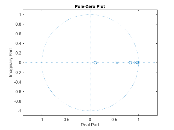
Generate samples of white Gaussian noise. Create a signal of pseudopink noise by filtering the white noise with a filter whose zeros and poles are all on the positive x-axis. Visualize the zeros and poles.
N = 1e5;
wn = randn(N,1);

z = [0.982231570015379 0.832656605953720 0.107980893771348]';
p = [0.995168968915815 0.943841773712820 0.555945259371364]';

[b,a] = zp2tf(z,p,1);
pn = filter(b,a,wn);

zplane(z,p)
Create a two-channel signal consisting of white and pink noise. Compute the octave spectrum. Assume a sample rate of 44.1 kHz. Set the frequency band from 30 Hz to the Nyquist frequency.
sg = [wn pn];

fs = 44100;

poctave(sg,fs,FrequencyLimits=[30 fs/2])
legend("White noise","Pink noise",Location="southeast")
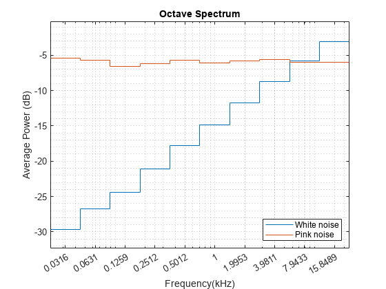
The white noise has an octave spectrum that increases with frequency. The octave spectrum of the pink noise is approximately constant throughout the frequency range. The octave spectrum of a signal illustrates how the human ear perceives the signal.
Generate samples of white Gaussian noise sampled at 44.1 kHz. Create a signal of pink noise by filtering the white noise with a filter whose zeros and poles are all on the positive x-axis.
N = 1e5;
fs = 44.1e3;
wn = randn(N,1);

z = [0.982231570015379 0.832656605953720 0.107980893771348]';
p = [0.995168968915815 0.943841773712820 0.555945259371364]';
[b,a] = zp2tf(z,p,1);

pn = filter(b,a,wn);
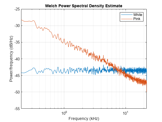
Compute the Welch estimate of the power spectral density for both signals. Divide the signals into 2048-sample segments, specify 50% overlap between adjoining segments, window each segment with a Hamming window, and use 4096 DFT points.
[pxx,f] = pwelch([wn pn],hamming(2048),1024,4096,fs);
Display the spectral densities over a frequency band ranging from 200 Hz to the Nyquist frequency. Use a logarithmic scale for the frequency axis.
pwelch([wn pn],hamming(2048),1024,4096,fs)
ax = gca;
ax.XScale = "log";
xlim([200 fs/2]/1000)
legend("White","Pink")
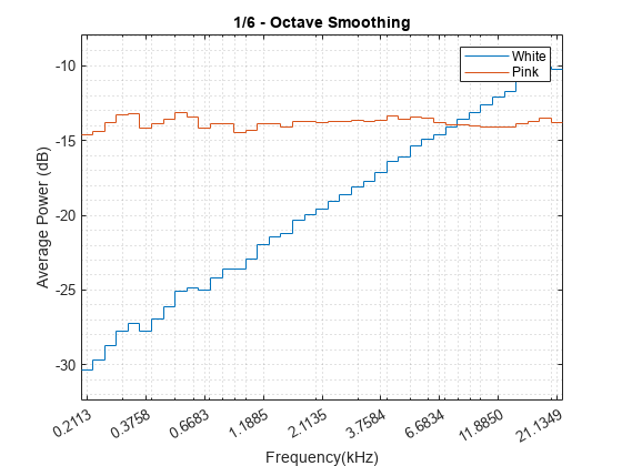
Compute and display the octave spectra of the signals. Use the same frequency range as in the previous plot. Specify six bands per octave and compute the spectra using 8th-order filters.
poctave(pxx,fs,f,"psd", ...
    BandsPerOctave=6,FilterOrder=8,FrequencyLimits=[200 fs/2])
legend("White","Pink")
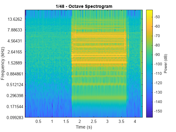
Read an audio recording of an electronic toothbrush into MATLAB®. The toothbrush turns on at about 1.75 seconds and stays on for approximately 2 seconds.
[y,fs] = audioread("toothbrush.m4a");Compute the octave spectrogram of the audio signal. Specify 48 bands per octave and 82% overlap. Restrict the total frequency range from 100 Hz to fs/2 Hz and use C-weighting.
poctave(y,fs,"spectrogram",BandsPerOctave=48, ...
    OverlapPercent=82,FrequencyLimits=[100 fs/2],Weighting="C")
Generate samples of white Gaussian noise sampled at 44.1 kHz. Create a signal of pink noise by filtering the white noise with a filter whose zeros and poles are all on the positive x-axis.
N = 1e5;
fs = 44.1e3;
wn = randn(N,1);

z = [0.982231570015379 0.832656605953720 0.107980893771348]';
p = [0.995168968915815 0.943841773712820 0.555945259371364]';
[b,a] = zp2tf(z,p,1);

pn = filter(b,a,wn);
Compute the octave spectrum of the signal. Specify three bands per octave and restrict the total frequency range from 200 Hz to 20 kHz. Store the name-value pairs in a cell array for later use. Display the spectrum.
flims = [200 20e3];
bpo = 3;
opts = {"FrequencyLimits",flims,"BandsPerOctave",bpo};

poctave(pn,fs,opts{:});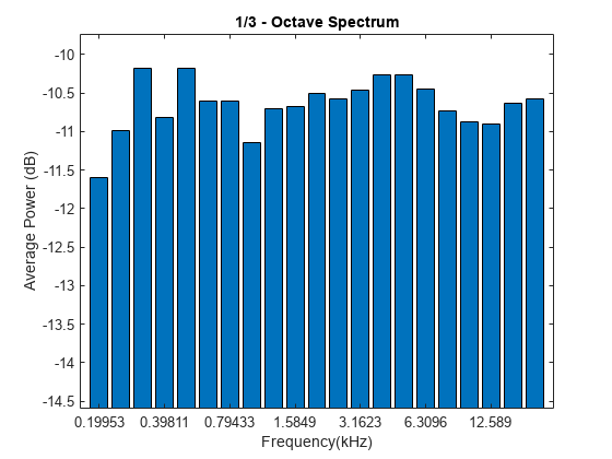
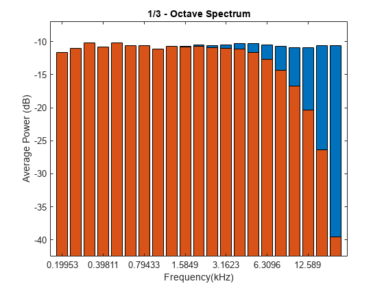
Compute the octave spectrum of the signal with the same settings, but use C-weighting. The C-weighted spectrum falls off at frequencies above 6 kHz.
hold on
poctave(pn,fs,opts{:},"Weighting","C")
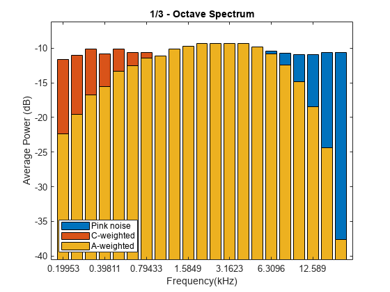
Compute the octave spectrum again, but now use A-weighting. The A-weighted spectrum peaks at about 3 kHz and falls off above 6 kHz and at the lower end of the frequency band.
hold on
poctave(pn,fs,opts{:},"Weighting","A")
hold off
legend("Pink noise","C-weighted","A-weighted","Location","SouthWest")
Since R2026a
Plot the octave spectrum and octave spectrogram for four signals in the specified target axes and panel containers.
Create four oscillating signals with a sample rate of 10 kHz for three seconds.
Fs = 10e3;
t = 0:1/Fs:3;
x1 = vco(sawtooth(2*pi*t,0.5),[0.1 0.4]*Fs,Fs);
x2 = vco(sin(2*pi*t).*exp(-t),[0.1 0.4]*Fs,Fs) ...
    + 0.01*sin(2*pi*0.25*Fs*t);
x3 = chirp(t,Fs/10,t(end),Fs/2.5,"quadratic");
x4 = cos(pi*sin(4*t)*Fs/10);
Plot Octave Spectra in Target Axes
Create two axes in the southwestern and northeastern corners of a new figure window.
fig = figure;
ax1 = axes(fig,Position=[0.10 0.3 0.35 0.56]);
ax2 = axes(fig,Position=[0.55 0.7 0.42 0.25]);
Plot the octave spectra of the signals x1 and x2 in the southwestern and northeastern axes of the figure, respectively.
The octave spectrum of
x1uses six bands per octave and 8th-order filter.The octave spectrum of
x2uses"A"frequency weighting.
poctave(x1,Fs,BandsPerOctave=6,FilterOrder=8,Parent=ax1)
poctave(x2,Fs,Weighting="A",Parent=ax2)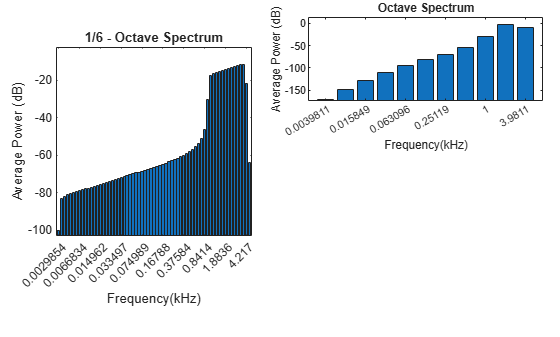
Plot Octave Spectrum in Target UI Axes
Create an axes in the northwestern corner of a new UI figure window.
uif = uifigure(Position=[100 100 720 540]);
ax3 = uiaxes(uif,Position=[5 305 300 200]);
Calculate the Welch power spectral density of x3 and plot its octave spectrum in the figure axes. Use a 2048-sample Hamming window, 1024 overlapping samples between adjoining segments, and 4096 DFT points.
[pxx3,f3] = pwelch(x3',hamming(2048),1024,4096,Fs);
poctave(pxx3,Fs,f3,Parent=ax3)
title(ax3,"Octave Spectrum in UI Axes")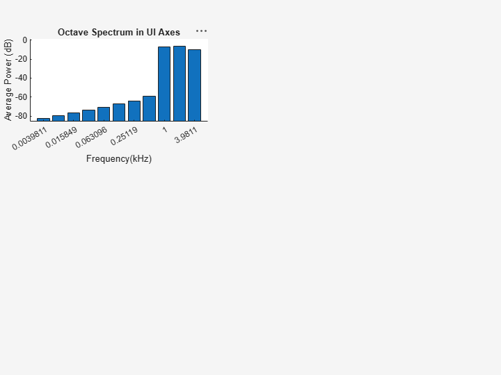
Plot Octave Spectrogram in Target Panel Container
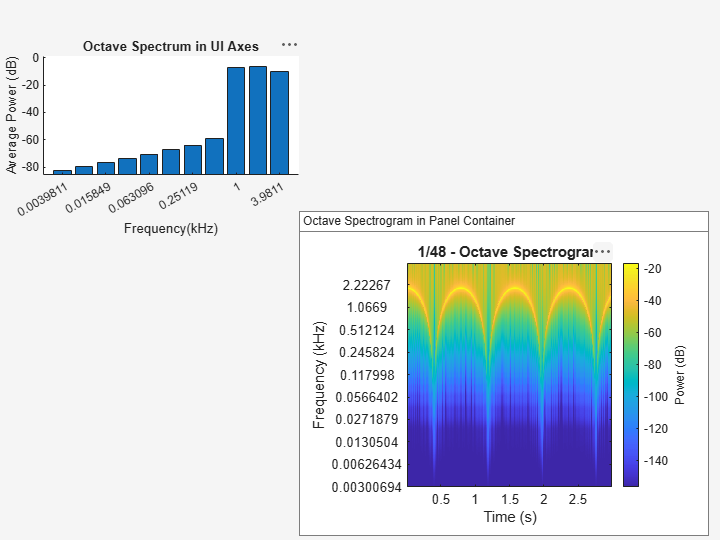
Add a panel container in the southeastern corner of the UI figure window.
p = uipanel(uif,Position=[300 5 410 325], ...
    Title="Octave Spectrogram in Panel Container", ...
    BackgroundColor="white");
Plot the octave spectrogram of the signal x4 on the panel container. Use 48 bands per octave, 82% overlap, and "C" frequency weighting.
poctave(x4,Fs,"spectrogram",BandsPerOctave=48, ...
    OverlapPercent=82,Weighting="C",Parent=p)
Input Arguments
Name-Value Arguments
Output Arguments
Algorithms
References
[1] Smith, Julius Orion, III. "Example: Synthesis of 1/F Noise (Pink Noise)." In Spectral Audio Signal Processing. https://ccrma.stanford.edu/~jos/sasp/.
[2] Specification for Octave-Band and Fractional-Octave-Band Analog and Digital Filters. ANSI Standard S1.11-2004. Melville, NY: Acoustical Society of America, 2004.
[3] Orfanidis, Sophocles J. Introduction to Signal Processing. Englewood Cliffs, NJ: Prentice Hall, 2010.